Algebra of Matrices Systems of Linear Equations
5. Systems of linear equations II: Rouché-Capelli's
theorem and
Cramer's theorem
Rouché-Capelli's theorem provides a useful tool to determine whether a system is
solvable or not .
Theorem 4 (Rouché-Capelli). Let AX = b be
 . Such LS is
solvable if and only if rank (A) = rank (A b).
If such system is solvable, then it admits  solutions.
Proof. AX = b is solvable  there
exists
such that Aa = b
there
exists
such that Aa = b
there exists 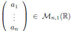 such that
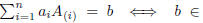

rank (A b).
Now, suppose that the LS(m, n,R) AX = b is solvable and denote r = rank (A) =
rank (A b). Without any loss of generality (up to interchanging the rows of A),
we
can assume that the first r rows of A are linearly independent . Therefore, also
the
first r rows of (A b) are linearly independent (and the remaining m−r are a
linear
combinations of the former ).
Let us denote:
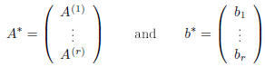
and consider the LS(r, n,R) A * X = b* . It is easy to see
that this LS is equivalent
to the original one; hence, we will solve A *X = b* , instead of AX = b.
If we apply the Gauss-Jordan algorithm to A *X = b* , since this system is
compatible,
we will end up with a step LS ; moreover, since rank (A) = r and the rank is
preserved by elementary operations, we won't obtain any zero row! In the end our
step system will have exactly r equations and , as observed in prop. 6, it will
have
 .
.
Proposition 9. Let
![]() and
and
![]() . One has:
. One has:
rank (AB) ≤ min{rank (A), rank (B)}.
Proof. It is sufficient to verify that rank (AB) ≤rank (B). In fact, if this
inequality
is true, it follows that:

Let us consider the i-th row of AB:
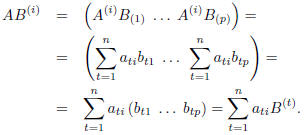
Therefore,  . It follows
that
. It follows
that

and consequently rank (AB) ≤ rank (B).
Corollary 2. Let ![]() .
For any
.
For any  and
and
 , one
, one
has:
rank (A) = rank (AB) = rank (CA).
Proof. We have: rank (AB) ≤ rank (A) = rank (ABB -1) ≤ rank
(AB); therefore,
rank (AB) = rank (A) .
Analogously: rank (CA) ≤ rank (A) = rank (C-1CA) ≤ rank (CA);
therefore,
rank (CA) = rank (A) .
Let us state and prove another method , that can be used to solve LS(n, n,R):
Cramer's method.
Theorem 5. Let AX = b a LS(n, n,R), with
![]() . We have:
. We have:
i) this LS has a unique solution;
ii) for i = 1, . . . , n let us denote with  the matrix obtained by A, substituting
the i-th column ![]() with
b. The unique solution of this LS is given by:
with
b. The unique solution of this LS is given by:
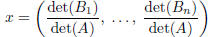
(Cramer' s formula ).
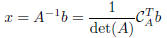
Proof. i) The column x = A-1b is a
solution of AX = b; in fact:

If y is another solution, then:

therefore, the solution is unique.
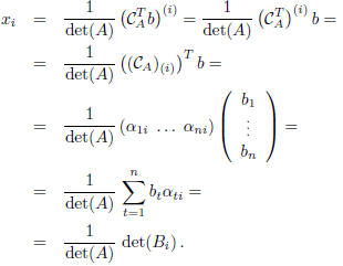
ii) Let us compute the determinant of
![]() , using Laplace's
expansion (cofactors
, using Laplace's
expansion (cofactors
expansion) with respect to the i-th column:
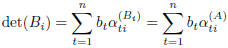
[in fact, the cofactors w.r.t. the i-th column of A and B
coincide].
Since 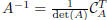 , then
and consequently (for i = 1, . . . , n):
From Rouché-Capelli's theorem, it follows that, in order
to decide whether a LS
AX = b is solvable or not, one has to compute ( and then compare ) rank (A) and
rank (A b).
To compute the rank of a matrix, the following result (Kroenecker's theorem or
theorem of the bordered minors) will come in handy, saving a lot of
computations!
Let us start with a Definition.
Definition. Let B be a square submatrix of order r, of a matrix
![]() .
.
We will call a bordered minor of B, the determinant of any square submatrix C of
A, of order r + 1 and such that it contains B as a submatrix. We will say that C
is obtained by bordering B with a row and a column of A.
Obviously, if r = min{m, n} B has no bordered minors.
Theorem 6 (Kroenecker). Let
![]() . We have that rank
(A) = r if and
. We have that rank
(A) = r if and
only if the two following conditions are satisfied:
a) there exists in A an invertible square submatrix B of order r;
b) all bordered minors of B (if there exist any) are zero .
Proof. (=>) If rank (A) = r, then
![]() (A) = r and therefore
there exists an invertible
(A) = r and therefore
there exists an invertible
submatrix of A of order r:  . Moreover, all
minors of order
. Moreover, all
minors of order
r + 1 of A (and in particular the bordered minors of B) are zero. Hence,
conditions a) and b) are satisfied.
( ) To simplify the
notation , let us suppose that B = A(1, . . . , r | 1, . . . , r). By
) To simplify the
notation , let us suppose that B = A(1, . . . , r | 1, . . . , r). By
hypothesis, det(B) ≠ 0 (i.e., rank (B) = r).
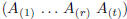
Let C = ( ) be the submatrix of A, formed by
the first r columns
) be the submatrix of A, formed by
the first r columns
of A. Obviously, rank (C) ≤r; since B is a submatrix of C, then r =
rank (B) ≤rank (C) ≤ r and consequently, rank (C) = r. Hence, the
columns are linearly independent.
To show the claim (i.e., rank (A) = r), we need to prove that:

namely, that for t = r + 1, . . . , n, the matrix
 has rank
r.
Let us denote such matrix by 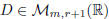 and consider
the submatrix
and consider
the submatrix
formed by the first r rows:
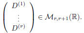
This submatrix has rank r (it has B as a submatrix,
therefore it must have
maximal rank). To prove the claim (i.e., rank (D) = r), it suffices to verify:

In fact, for s = r + 1, . . . ,m, consider
 . This is a bordered
matrix of B, therefore it is zero. This means that its first r + 1 columns
are linearly dependent and, since the first r
 are linearly independent,
we have necessarily:
as we wanted to show.
Remark. Let ![]() .
To compute the rank one can proceed as follows:
.
To compute the rank one can proceed as follows:
• find in A an invertible square matrix B of order t;
• if t = min{m, n}, then rank (A) = t;
• if t < min{m, n}, consider all possible bordered minors of B;
• if all bordered minors of B are zero, then rank (A) = t;
• otherwise, we have obtained a new invertible square matrix C of order t+1;
• therefore, rank (A) ≥t + 1 and we repeat the above procedure.
Without Kroenecker's theorem, once we have found an invertible square submatrix
B of order t, we should check that all possible minors of order t + 1 are zero;
they
are  ; while the bordered minors of B are only
(m − t)(n − t).
; while the bordered minors of B are only
(m − t)(n − t).
For instance, if  and
and
 , the minors of A of order 3 are
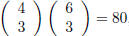 , while the bordered minors are (4 − 2)(6 −
2) = 8.
, while the bordered minors are (4 − 2)(6 −
2) = 8.
Remark. Let AX = b be a given LS(m, n,R). Let M = (A b) be its complete
matrix and let r = rank (A). From Rouché-Capelli's theorem, such LS is solvable
if and only if rank (A b) = r. In this case, it has
![]() solutions.
solutions.
We want to describe now a procedure to find such solutions
(without using Gauss-
Jordan's method).
Choose in A an invertible square submatrix B of order r (that we will call fun-
damental submatrix of the LS). For instance, let
 .
.
define:
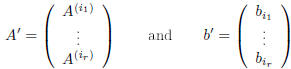
and consider the new LS(r, n,R): A'X = b'. This system is
equivalent to the original
one, since it has been obtained by eliminating m− r equations, corresponding
to the rows of A that could be expressed as linear combinations of the remaining
r.
Let us solve this new system. Bring the n−r unknowns different from

to the right-hand side and attribute to them the values
 (arbitrarily
chosen). We get in this way, a system LS(r, r,R) that admits a unique solution
(since the coefficient matrix B is invertible), that can be expressed by
Cramer's
formula. Varying the n − r parameters  , we
get the set
, we
get the set
![]() of the
of the
![]() solutions of the LS.
solutions of the LS.
A particular simple solution of the system, is obtained by choosing

 ; let us denote it by
 . Using prop. 5,
 (where
![]() denotes
denotes
the vector space of the solutions of A'X = 0); therefore, instead of computing
the
generic solution of , it might be more convenient to compute the generic
solution
of this HLS and then sum it up to .
Attributing to  the values,
(1, 0, . . . , 0), (0, 1, 0, . . . , 0), . . . , (0, . . . , 0, 1) ,
we get n − r systems LS(r, r,R), each of which admits a unique solution. These
n−r solutions  are linearly independent and
hence form a basis of
are linearly independent and
hence form a basis of ![]() .
.
Therefore:
Remark. We have already observed that a HLS AX = 0
is always solvable (in
fact, it has at least the trivial solution). This fact, is con rmed by
Rouché-Capelli's
theorem; in fact, rank (A) is clearly equal to rank (A 0). From the same
theorem,
it follows that every HLS(m, n,R) AX = 0 has  .
.
One can verify that a HLS has no eigensolutions (i.e., the only solution is the
trivial one), if and only if n = rank (A) [in fact,
 ].
].
| Prev | Next |