Conic Sections and Quadratic surface Lab

Goals

By the end of this lab you should:

1.) Be familar with the important features of ellipses and hyperbolas . For ellipses
these are the semi-major and semi-minor axes, for hyperbolas these are the vertices and
asymptotes.

2.) Understand the connection between the equation of the ellipse, and the length of
the semi-major and semi-minor axes.

3.) Understand the connection between the equation of the hyperbola and its vertices
and asymptotes.

4.) Be able to draw ellipses and hyperbolas whose equations are in standard form.
5) Be able to recognize the kind of quadratic surface defined by an equation from the
graph of the equation.

Introduction

Calculus is about functions. Some basic examples are linear functions like f(x, y) =
3x + 4y and quadratic functions like g(x, y) = 3x² + 4y² or h(x, y, z) = 3x² + 4y² − z².
Calculus is powerful, because it often reduces understanding a complicated function to
understanding a linear or quadratic one. Still, we have to understand the linear and
quadratic functions. In order to understand a quadratic function like g(x, y) = 3x² +4y²,
we have to understand its levels. These are the curves g(x, y) = c, and they are examples
of ellipses.

In the first two parts of this computer lab, we will review ellipses and hyperbolas. We
will need to be able to draw these curves so that we can draw level curves of quadratic
functions of two variables. It will turn out that the pattern of level curves around the
critical points of a function of two variables in “most” cases looks like a family of concentric
ellipses or hyperbolas.

Specifically, in this lab you will examine the equations of ellipses and hyperbolas in
standard form, see how the shape of the conic section is related to the terms of the equation ,
and review how to draw the graphs of the equations.

This should give you a good feel for quadratic functions in two variables. As a start
to understanding quadratic functions in three variables, in the third part of the lab, we
give you some practice recognizing some of the level sets of quadratic functions of three
variables.

This lab will also introduce you to the MAPLE software package, which is an extremely
powerful tool for doing mathematical calculations and graphing.

Background

As we all know, the equation x² + y² − 1 = 0 describes a circle in the xy-plane. In
general, quadratic equations of the form

Ax²+ Bxy + Cy² + Dx + Ey + F = 0

describe plane curves known as conic sections. For different choices of the constants
A, B, C, D, E, F you can get an ellipse, hyperbola, parabola , pair of lines, a single line or
a point as the graph of the equation. These sets are called conic sections because they are
the sets you can get if you intersect a cone with a plane.

Ellipses

The graph of the equation x²/a² + y²/b² = 1 is an ellipse in standard form. An
ellipse has two perpendicular lines of symmetry; for an ellipse in standard form these lines
of symmetry are the x and y axes. (We say a line L is a line of symmetry for a shape
if L divides the shape into 2 congruent pieces, and the two pieces match if we rotate one
around L.) Every ellipse has a major axis and a semi-major axis, a minor axis and a
semi-minor axis.

For an ellipse in standard form look at the part of the coordinate axes lying inside
the ellipse; the longer of the two segments is the major axis and the shorter is the minor
axis. The part of the major axis which runs from the center of the ellipse to the end of the
major axis is called the semi-major axis, while the part of the minor axis from the center
of the ellipse to the end of the minor axis is the semi-minor axis. In the graph below, the
semi-major axis lies on the y-axis and has length 2, while the semi-minor axis lies on the
x-axis and has length 1.

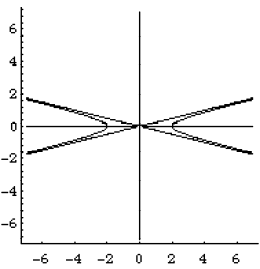
Hyperbolas
The graph of the equation x²/a²−y²/b² = 1 is a hyperbola in standard form. The
x and y axes are lines of symmetry for this shape. The hyperbola has two points which are
closest to the origin; these are called vertices, and they lie on the x-axis, if the hyperbola
is in standard form.

The hyperbola also has two asymptotes. The equations for the asymptotes are gotten
by taking the quadratic function x²/a² − y²/b², setting it equal to zero, factoring it, and
setting each factor equal to zero. The two equations for the asymptotes that we get are:

x/a + y/b = 0

and

x/a − y/b = 0

The figure below is a hyperbola, with vertices at (-2,0), (2,0) and with asymptotes 4y = x,
−4y = x. So that you can see how closely the hyperbola hugs the asymptotes, we have
included them in the figure.

Ellipses

Question 1.
(a) Plot x ²/a²+y² = 1 for a = 1, 3, 5, 7. We suggest you use a do loop of the following
form. (The MAPLE code is explained in the glossary just before the lab)

>with (plots);
>for a from 1 by 2 to 7 do
>implicitplot (x^2/a^2 + y^2=1,x=-8..8,y=-8..8,
scaling=constrained, axes=normal, grid=[100,100])
>od;

You may also use the following commands.

>with (plots);

>implicitplot ({seq(x^2/(2*j-1)^2 + y^2= 1, j=1..4)},
x=-8..8,y=-8..8,scaling=constrained, axes=normal,
grid=[100,100]);

These commands run faster, but they put all the plots in the same window, so you
should be sure you know which values of a go with which plots. Remember that a = 2*j−1.
Don’t print the plots unless you need to refer to them!

Describe the changes you see in the graph as the coefficient a increases. Say what
the length of the semi-major axis is for each value of a. What is the length of the
semi-minor axis?

(b) Plot x² + y²/b² = 1 for b = 1, 3, 5, 7.

Describe the changes you see in the graph as the coefficient b increases. What is
the length of the semi-major axis for each value of b? What is the length of the
semi-minor axis?

Question 2. What is an equation of an ellipse whose semi-major axis lies on the x-axis,
such that the semi-major axis is four times as big as the semi-minor axis?

Attach a print out of the graph of your ellipse. (Use the implicitplot command.)

Question 3. Plot x²/9 + y²/4 = c for c = −2, 0, 2, 4, 6.

Notice that the curves you just plotted are levels −2, 0, 2, 4, 6 of the function
f(x, y) = x²/9 + y²/4. As c increases, describe the changes you see in the plots.
Based on these plots, describe how the level curves of f change as c goes from
−∞ to ∞.

Hyperbolas

Question 4. Don’t print the plots unless you need to refer to them!

(a) Plot x²/a² − y² = 1 for a = 1, 3, 5, 7.

Describe the changes you see in the graph as the coefficient a increases. (Make
sure you mention how the asymptotes and vertices change. If you forget what the
asymptotes are or how to find their equations, look back at the bottom of page
5.)

(b) Plot x² − y²/b² = 1 for b = 1, 3, 5, 7.

Describe the changes you see in the graph as the coefficient b increases. (Make
sure you mention how the asymptotes and vertices change.)

Question 5. Find the equation of a hyperbola whose asymptotes have slope 1 and −1,
and whose vertices are located at (−6, 0), (6, 0).

Attach a printout of the graph of your hyperbola.

Question 6. Plot x² − y² = c for c = −16,−4, 0, 4, 16.

Describe the changes you see in the plots as the coefficient c increases. Notice
that the curves you just plotted are levels c = −16,−4, 0, 4, 16 of the function
f(x, y) = x²−y². Based on these plots, describe how the level curves of f change
as c goes from −∞ to ∞.

Recognizing Quadric Surfaces

If we have a quadratic equation of three variables, like 2x² + x − z − xy + 2yz = 1
it’s often hard to see what kind of surface it defines by looking at the equation. (If you go
on in linear algebra you will learn a way to tell which kind of surface you have from the
equation in that subject.) However, with a little practice we can use a plotting program
like Maple to help us with the identification.

Use Maple and implicitplot3d to identify the surfaces given by the equations below.
In each case attach a printout of the plot, and give the name of the surface (for example,
“Hyperboloid of 1 sheet”). At least for starters, include the following commands x=-3..3,
y=-3..3, z=-3..3, axes=boxed, grid=[12,12,12]. Once you get a plot, you may want
to change some or all of these. Remember that you can also rotate the plot to get a better
viewpoint: click on it once so that a frame forms around it (this will also give various
plotting options on the menu bar at the top of the screen); now dragging the plot in
various directions will cause it to rotate. Do this slowly and carefully; it takes a while to
get used to how it works.

Finally, you can probably fit at least two of these plots on a page: this will save time
and paper!