FINITE MATHEMATICS: ACTIVITY
Systems of Linear Equations
This sheet includes only instruction sections. Please work through the
instructions. Turn in a printout
of each of your completed worksheets in the spreadsheet. There should be four
complete worksheets in all.
Introduction. In this activity we’ll learn how to use a spreadsheet to
solve linear systems via the Gauss-
Jordan elimination method introduced earlier in the week. As you may have
noticed, solving 3 × 3 systems
by hand can become quite laborious fairly quickly. Imagine having to solve a 5 ×
5 system by hand or a
10 × 10.
Required Problems (To be turned in)
Solving a 2 × 2 System.
A. Open the spreadsheet gaussian.xls which is posted on the class web site.
It may be easiest to save
it first and then open it in Excel rather than opening it directly in the
browser. If you do have to
open it within the browser, you will probably want to copy the data into a
stand-alone Excel session,
rather than working within the browser.
B. Make sure you’re in the 2×2 worksheet. We’re going to solve the 2×2 system
in Example 4 on page
81 in your text first to see how things work. Then we’ll work on larger systems
later on. You should
see an array of numbers representing the augmented matrix given in Example 4.
C. Our first row operation will be R1->R2-> R1, so we get 1 in the top left
component of the augmented
matrix. We’ll do this in the following steps.
i Click and drag to select cells A5..C5 (this will be the new R1).
ii Click in the top formula input bar (next to the fx).
iii Type = (while still in the formula input bar).
iv Click and drag to select cells A2..C2 (this is R1).
v Your cursor should be in the formula input bar. Type −.
vi Click and drag to select cells A3..C3 (this is R2)
vii Type CTRL-SHIFT-ENTER (This means hold down the CTRL key with one
finger, hold down
the SHIFT key with another finger and then hit ENTER with third finger).
viii You should get a new R1 that looks like 1 2 4.
ix Copy cells A3..C3 to A6..C6.
D. The next row operation is −2R1 + R2 -> R2, so we get 0 in the lower left
corner.
i Select cells A8..C8, type = in the formula bar, select cells A5..C5 and
type CTRL-SHIFT-
ENTER. We just copied cells A5..C5 to A8..C8 (this will be R1). The standard
copy and paste
doesn’t work here since we’re using formulas. Try and it and see.
ii Select cells A9..C9, type = in the formula bar, select cells A6..C6,
type − in the formula bar,
select cell A6, type * in the formula bar, select cells A5..C5 and type
CTRL-SHIFT-ENTER.
iii You should get a new R2 that looks like 0 -1 -3.
E. It should be obvious what row operation you should probably do next. Use a
similar technique to
part D to eliminate the 2 in the top row. Compare your answer with the one given
in Example 4,
page 81 in the book.
Solving a 3 × 3 System. Now we solve a 3 × 3 system using similar
techniques as above, but we’ll learn a
new trick to speed things up a tiny bit.
F. Go to the 3×3 worksheet. You should see a representation of the augmented
matrix from the system
in Exercise 2.24 from the Class Notes that you did earlier in the week.
G. Do the row operation R1 <-> R2. A standard copy and paste should work,
since we haven’t used any
formulas yet. Make sure your top row has a 1 in the left corner and is in cells
A7..D7.
H. Here, we’ll do two row operations at once, −2R1+R2 and −3R1+R2 using the
drag feature in Excel.
Complete the following steps:
i Copy and paste the top row of the given matrix into cells A11..D11 (R1
won’t change).
ii This step is similar to Step ii in Part D. Select cells A12..D12, type
= in the formula bar, select
cells A8..D8, type − in the formula bar, select cell A8, type * in the formula
bar, type A$7:D$7
and type CTRL-SHIFT-ENTER.
Note that the numbers without $ signs in front of them are “relative cell
references”, which will
be automatically adjusted when the formula pasted or dragged. The numbers with $
signs in
front of them are “absolute cell references”, which are not changed when the
formula is pasted
and dragged somewhere else.
iii Select cells A12..C12, then click on the bottom right corner and drag
the box down so cells
A13..D13 are also selected. You just did the −3R1 + R2 row operation.
H. Continue row reducing the matrix and compare your solution to the one we did in the previous class.
Solving a 5 × 5 System.
I. Solve the 5 × 5 system in the 5 × 5 worksheet (not the 5 × 5 Reprise worksheet).
J. Go to the 5 × 5 Reprise worksheet tab. We’re going to solve this system
using a different technique
that we’ll learn in Section 2.6. This problem is Technology Exercise 5, Page 91
in your text. We can
represent the linear system in this problem by the following matrix equation :
which is of the form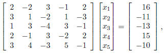
Ax = b.
If we multiply the matrix A by x and set it equal to b, we get the system
given in the problem. We
can “undo” the matrix A by multiplying A by its inverse A-1. That is,
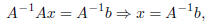
which means we have a way to solve for x. We will actually
learn how to do matrix multiplication
and how to find a matrix inverse next week, but for now we’ll let the
spreadsheet do it for us.
K. We’ll solve the system in the following steps:
i We’ll have Excel compute the inverse of A. Select
cells B17..F21, type =MINVERSE(B10:F14)
in the formula input bar and type CTRL-SHIFT-ENTER. Cells B10..F14 give the
matrix A.
ii Now we can solve for x = A-1b by having Excel multiply
matrix A-1 by matrix b. Select
cells B24..B28, type =MMULT(, select cells of matrix A-1, type a
comma, select the cells of
matrix b and type ). Your formula should look like =MMULT(B17:F21,I10:I14).
Finally type
CTRL-SHIFT-ENTER. You should now have the correct solution .
| Prev | Next |