Math 256 Study Guide
Chapter 1: Introduction
• Draw direction fields for differential equations of the form y' = f(t,
y) (1.1).
• Understand the definition of general solution and particular solution
(1.2, 1.3).
• Be able to show given functions are solutions to differential equations
(1.3).
• Classify differential equations by order and linearity (1.3).
Chapter 2: First order differential equations
• Solve first order linear differential (y' + p(t)y = g(t)) using
integrating factors 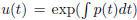
(2.1).
• Write solutions in terms of definite integrals if needed (2.1).
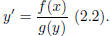
• Solve first order nonlinear equations by separation. Separable
differential equations are of the form
• Use differential equations to answer modeling questions (Tank problems
and interest problems in 2.3).
• Understand when solutions are guaranteed to exist and be unique for
linear and nonlinear equations
(2.4).
• Understand what types of behavior solutions may exhibit if solutions are
not unique (2.4).
• Graph solutions to autonomous equations (y' = f(y)) using the graph of
"y versus f(y)" and without
solving for explicit solutions (2.5).
• Understand equilibrium solutions and determine if they are stable,
unstable or semi-stable (2.5).
• Determine if a differential equation is exact and find solutions to
exact equations. Exact equations are
of the form M(x, y) + N(x, y)y' = 0 where  (2.6).
• Approximate solutions to differential equations of the form y' = f(t, y)
using Euler's method. Euler's
method uses the equation of a tangent line and the process given by the
recursive formula
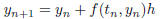
where h is a fixed differential (2.7).
Chapter 3: Second order differential equations
• Find general and particular solutions to second order, homogeneous,
linear equations with constant
coefficients (ay'' + by' + cy = 0) (3.1, 3.3, 3.4). In order to find solutions
we look at the characteristic
equation ar2 +br +c = 0. The roots of the polynomial determine the
form of the solutions. The three
cases are:
1.  , both real .
2.  are complex .
3.  , both real.
• Compute the Wronskian of two functions and understand the connection to
fundamental sets of solu-
tions to second order linear homogenous equations (3.2).
• Understand when solutions are guaranteed to exist and be unique for
linear second order differential
equations (3.2).
• Find particular solutions to nonhomogeneous equations using the method
of undetermined coefficients
(3.5). The types of functions covered are:
1. Exponentials : 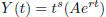 .
.
2. Sine and cosine:  .
.
3. Polynomials:  .
.
and all combinations of products and sums of these functions. The variable s =
0, 1, or 2 depending
on the roots of the characteristic equation.
• Find general solutions to nonhomogeneous equations using solutions to
homogeneous equations (y =
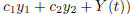 (3.5).
Chapter 4: Higher order differential equations
• Understand how the techniques used to study second order linear
differential equations extend to higher
order differential equations (4.1).
• Compute the Wronskian of three or four functions (4.1).
• Find general and particular solutions to higher order, homogeneous,
linear equations with constant
coefficients. There equations are of the form 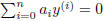 (4.2).
• Find roots to characteristic polynomials using long division .
• Find roots to characteristic polynomials using Euler's equation
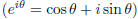 (4.2).
• Find particular solutions to nonhomogeneous equations using the method
of undetermined coefficients
for higher order differential equations (4.3).
Chapter 7: Systems of differential equations
• Solve systems of two first order differential equations by rewriting the
system as single second order
equation (7.1).
• Write a system of differential equations as a single higher order linear
differential equation (7.1).
• Write a linear differential equation (of order ≥ 2) as a system of
first order differential equations (7.1).
• Add , multiply and scale matrices (7.2).
• Write systems of differential equations in matrix form (7.3).
• Solve a given system of linear equations using row reduction of matrices
(7.3).
• Find eigenvalues and eigenvectors of square matrices (7.3).
• Write solutions to differential equations in vector form (7.2, 7.4).
• Compute the Wronskian of a system of solutions (7.4).
• Find solutions to systems of differential equation using eigenvectors
and eigenvalues (7.5).
| Prev | Next |