Some Advice on TI-89 Functions for Calculus II

General Remarks

The Catalog key provides the user with a list of all built-in functions on the TI89, complete with instructions. (Look at the
very bottom of the screen when you get to the function you want.) When you press the Catalog key, you put the keyboard
into Alpha mode. To find a function you want after pressing Catalog, for example Limit, press the key corresponding to the
first letter of the function. In our example, we would press 4 and that would put us at the top of the list of functions that
start with the letter L.

If you are in the midst of using an unfamiliar function, and you need a reminder as to how to use the function, press the
Catalog key again, scroll to the function, look at the bottom of the screen, then hit ESC.

You may access functions via menus, the Catalog, or by typing them in by hand.

Clear everything before you start on a new problem. A way to do that is to clear the command line (where you input
commands), then access the NewProblem function (F6, 2, Enter). This clears all single letter entries in memory so that if
you talk to the calculator about a , it will not know what you mean until you give it instructions as to how to interpret a.
NewProb does not clear the memory of anything but the history (the last 30 lines) and single letter assignments. It does
deselect what is on the current Y= menu, but it does not erase the functions on your list. (If you are in Function mode, for
example, any selected functions on your Parametric or Polar lists are unaffected.)

Failure to start with NewProblem is a common source of errors. Get into the habit of using NewProblem right away and
remind students of it early and often.

Do not use implicit multiplication with the TI89. If you try talking to it about 2 sin(x), for example, it will think that
2 sin is a variable name . You must type 2 × sin(x) if you mean 2 sin(x). Get into that habit right away and remind students
of it early and often.

Use Second, scroll down arrow, to scroll to the top of the next screen. Use green diamond, down arrow, to get to the
bottom of a list. These work when you are scrolling through the catalog, a menu, or the history screen.

The TI-89 has many editing features we use on the computer. The arrow key next to the Second key is for upper case.
Use it with the scrolling keys to highlight so that you can then cut and paste.

If you work a multistep problem on the TI-89 and you want to save the steps, hit F1, 2, and give it a variable name. This
will save your steps as a text file. To access that file, hit APPS, 8, 2, then find your file name on the menu next to Variable.
Note that when you acquire a long list of text files, you can jump closer to what you want on the list by typing the first letter
of the file name you want. (Note, the keyboard is in alpha mode so do not press the alpha key first.) To invoke the steps
of the problem, in other words, to get your home screen to look as it did when you saved the problem originally, you must
execute the commands in the text file. Do that by mashing F4 on each line that starts with C:

Chapter 5

Calculator functions that come up in these sections are: graphing, differentiation, antidifferentiation, evaluating logarithms
and exponentials , finding inverse functions. Other calculator versus pencil and paper calculation issues arise in logarithmic
differentiation and the formulas for derivatives of log_a(x) and a^x.

Graphing

The new feature here is ZoomFit. It is item 9 on the Zoom menu. This will often, but not always, allow you to get a decent
picture without setting the window yourself.

Logarithms
The TI-89 does not have a built-in feature for logarithms with arbitrary base. If you type ”Define loga(a,x)=ln(x)/ln(a),
Enter” you can use your new function to bypass the log conversion formula.
If you have variables like loga , text files, and programs that you do not want to lose or foul up, you should lock them. To
lock user-defined functions, press Second, −, to access the Variable Link screen, select the items you want to lock, then hit
F1, 6.

Differentiation and Integration
Differentiation is Second, 8. If you access it via the Catalog, you can see a note for the required syntax at the very bottom of
your screen. Antidifferentiation is Second, 7. You can also antidifferentiate via desolve(. (See the catalog for syntax.) When
you use desolve, you do get a constant of integration. The symbol for the constant looks strange. You can see that symbol
by typing Green Diamond, STO. The TI-89 keeps track of the number of constants that come up during its travels and it
numbers them.

Inverting Functions

Students can find the inverse of a function on the TI-89 by switching the independent and dependent variables and solving
for the independent variable. (Get solve( from the catalog to see the syntax.)

The calculator will provide the graph of the inverse of a given function: from the graphing window select F6, 3, then type
y1(x), if the function you want to invert is y1. The picture looks best with a square window .

Students must know that the calculator connects dots when it graphs and they must understand the ramifications when
it comes to vertical asymptotes and points of discontinuity in general. The students should know how to control the style of
a graph: pick your graphing style from the Y= screen by selecting F6.

Bases Other Than e and Other Sticking Points

The Committee recommends allowing students to have the formula 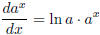or letting them use the calculator to get
that formula. On the other hand, we do recommend that students be instructed to perform logarithmic differentiation by
hand when they are told that logarithmic differentiation is called for. We are keeping that in the syllabus because it comes
up again, after a fashion, in L’Hopital’ s Rule .

See remarks above concerning calculations with log_a(x). The Committee is divided as to whether to insist that students
memorize the differentiation formula for log _a(x), or be able to derive it once they are given log_a(x) = lnx/ ln a.

We are putting in an optional section on hyperbolic trigonometric functions as they are ubiquitous in engineering applications
and also figure prominently in calculation algorithms. Some problems on hyperbolics show up in later assignments.
They should be marked optional but some may have snuck into the regular pool so keep an eye out for them if you want to
skip hyperbolics.

Chapter 7

Teaching this material with the calculator will allow us to streamline certain topics. Our recommendation is to spend more
time on straight substitution and integration by parts than on the other techniques of integration we usually teach. We are
not excising any of the techniques of integration from the course entirely, with the exception of integration by tables (see
remarks below.)

Calculator functions that come up in this chapter are integration, differentiation, limits, graphing.

Note that students do need some practice in using the calculator to do integration. Note, too, the calculator does not
always give the expected result and two TI -89s with the same settings will sometimes give answers that look different.

We have chosen very few problems that give the students nothing more than practice in pushing buttons. For more
practice in using the machine, students should check answers to the even numbered problems with the calculator. If the
students’ answers differ from the machine’s answer, the students should check with solve(, test equality of the two answers
with =, differentiate their result with the calculator if it’s too tedious to do by hand, etc. In short, students should develop
some facility in “torturing” the machine to give them what they want.

Integration by Tables
We recommend abandoning integral tables. We left this section in the syllabus to give us a day of applications problems.

Indeterminate Forms and L’Hopital’s Rule

The calculator can do some improper integrals. In cases where it balks, try doing the calculation the usual way with the
help of the machine: ask it for for example, and then ask it for the limit of the answer as h → ∞. A bit of
simplifying between the antidifferentiation and the limit can help out in some of these problems.

Chapter 8

Calculator functions that come up in this chapter are graphing in sequence mode, the Seq( command, summing (the command
is Σ(; see the catalog for the syntax), and Taylor(, the command for obtaining Taylor polynomials.

Graphing in Sequence Mode

Choose Sequence on the top line of the Mode menu. Press the Y= button. On the top line, you can enter a function of n to
graph a sequence such as 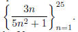You can enter a sequence that is defined iteratively. The first term is entered as
on the second line in the Y= menu.

Graphing the first several terms in a sequence of partial sums can give the students suggestions as to what goes on for
some series. For example, entering Σ(1/k, k, 1, n) for u1, and setting n and x to range from 1 to 50, y to range from 1 to 5,
the students can see that the graph of the harmonic series looks much like the graph for the natural logarithm.

Graphing two sequences together gives students a handle on the idea of comparing sequences .
Using the graph with the table feature allows students to explore sequence limits effectively.
Be sure to keep these devices in mind as you teach series as well.

The Sequence Command

The syntax seq(n!/(n + 1)!, n, 1, 19, 1) produces the first 19 terms of the sequence (Green Diamond, ÷
produces the factorial symbol.) The last argument in the seq command is the step size.

The Summing Command
Using the summing command and the sequence command together can give students as many terms as they like in a sequence
of partial sums. Use the syntax seq(Σ(1/n,n,1,k),k,1,25,1) to get the first 25 terms in the sequence of partial sums for
Summing and sequence graphing can be used together to similar effect.

The quickest way to accesst the summing command from the home screen may be from the Calculus menu, F3

Taylor
The Taylor command produces a Taylor polynomial of desired ordere centered at the desired point. See the Catalog for
syntax.
The machine crunches the numbers in the coefficients so the students will not see coefficients that look like for example.
The display shows the polynomial written with the term of highest degree first.

Use Taylor and function graphing together to get students to graph several Taylor polynomials for a given function at a
given point so that they can see convergence on an interval.

Chapter 9

We recommend a light treatment of parametric equations and polar graphing.
The calculator functions that come up in this chapter are parametric and polar graphing modes, integration, differentiation.
Note that we are covering arclength in parametric and area in polar. Both topics get a very light treatment with easy
homework problems. If you allow the students to get the derivatives and integrals using the calculator, it makes the problems
even easier.
The calculator does have an arclength function that works for rectangular. Joe Fadyn has a function that will find
arclength in the parametric case. (Note that once you have parametric, you get polar for free: that point should be stressed
for the students.)

When students are using the calculator to help with the calculation of an arclength, they will find out pretty fast that
the machine does not like grinding through the arclength formula in one shot. In other words, calculate dy/dt, dx/dt first.
Then find 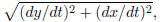then find the integral.