Linear Equations in Linear Algebra

Operations on a System of Linear Equations

Operations on a system of linear equations which do not change its set of solutions:
(1) multiply an equation by a scalar (number)
(2) replace an equation by the sum of itself and a scalar multiple of another equation
(3) interchange two equations

Elementary Row Operations on a Matrix

A system of linear equations can be represented by a matrix. Operations on the equations correspond to
elementary row operations on its matrix.
(1) multiply a row by a scalar ( number )
(2) replace a row by the sum of itself and a scalar multiple of another row
(3) interchange two rows

Definitions

(a) pivot
First non-zero entry in a row.
(b) echelon form
Each pivot occurs to the left of all pivots below it.
Any zero row occurs below all non-zero rows.
(c) reduced echelon form
Each pivot is 1.
Each pivot is the only non-zero entry in its column.

Algorithms for Solving a System of Linear Equations

(a) Gauss-Jordan
Use Gaussian elimination to arrive at the reduced echelon form of the matrix.
(b) Gaussian Elimination with Back- Substitution
Use Gaussian elimination to arrive at an echelon form of the matrix, then use back-substitution.

Case Study: Linear Models in Economics

Download the supporting pdf file and Mathematica notebook from the Lay Linear Algebra web site.

An Algebraic Point of View

Consider the set of all systems of linear equations with real coefficients having m equations and n
unknowns . Declare one such system to be equivalent to another if there is a sequence of elementary operations
(scale, swap, or replace) which transform the first into the second. This relationship is an equivalence relation,
and the solution set of such a linear system of equations is an invariant of its equivalence class. This is just
another way of saying that any two systems of linear equations which are equivalent to each other have the
same solution set.

Now consider the set of m by n+1 matrices with real coefficients . Declare one such matrix to
be equivalent to another if there is a sequence of elementary row operations which transforms the first into
the second. This defines an equivalence relation on this set of matrices, viewed as augmented matrices of
linear systems, so that these matrices break up into equivalence classes.

The map which sends a system of linear equations to its augmented matrix
is a bijection, and it respects equivalence classes. Thus, implies that
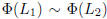, where the first is an equivalence of linear systems and the second is an equivalence of
augmented matrices. It works the other way as well, since elementary operations are invertible and their
inverses are other elementary operations. Thus, if two augmented matrices are equivalent, then the linear
systems they represent are also equivalent, and therefore they have the same solution sets.

This is the fundamental fact behind our interest in echelon forms and the like . They classify matrices, and
hence classify linear systems, in a manner which is invariant over equivalence classes, hence invariant over
solution sets. The following example illustrates this sort of relationship.

Suppose that a certain matrix A is equivalent to the reduced echelon matrix U, and it is clear by inspection
that the third column of U is a linear combination of its two previous columns. Then the third column of
A is also a linear combination of its two previous columns, because the related linear systems have the same
solutions. In fact, the coefficients which express this linear dependence are the same since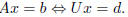

For a specific example of this sort of thing, consider that

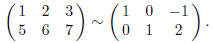
It is clear that the third column of the matrix on the right is a linear combination of the previous two columns.
Indeed, as well, since the vector x = (−1, 2,−1) is a
solution of both associated linear systems: Ax = 0 and Ux = 0.

Exercises

We will solve some of the following exercises as a community project in class today. Finish these solutions
as homework exercises, write them up carefully and clearly, and hand them in at the beginning of class next
Friday. You are encouraged to use a computer algebra system whenever appropriate.

Exercises for Lay, Section 1.1, pp 11–13: 1, 3, 5, 9, 13, 15, 33, 34 (heat transfer)
Exercises for Lay, Section 1.2, pp 25–27: 1, 3, 7, 11, 13, 17, 19, 33 ( interpolating polynomial ),
34 (wind tunnel experiment)