PROBLEM #6: WAGE DIFFERENTIALS
Introduction
When one looks at the labor market, one sees that not all jobs pay the same
wage, nor do
all individuals earn the same wage, even when they hold the same job. Wages vary
for
numerous reasons, including job characteristics, the amount of education and
training
required, the industry and region of the country in which they occur, and
whether the
work force is unionized of not. Wage differentials between jobs is a powerful
mechanism
in the allocation of labor, as higher paying jobs tend to be more attractive to
workers than
lower paying jobs. Where shortages of workers exsist, employers often raise
wages in
order to attract more workers. However, there also appears to be wage
differentials that
are associated with race or gender of the workers involved, and not with the
characteristics of the job or the qualifications of the worker.
In this section we will calculate some of these wage differentials.
Mathematics: Comparing Two Functions
If  and
and are two functions of x , then we may graph both functions
on the same set of axes. This enables us to compare the two functions . Some
questions
we might ask are:
1. When is ?
?
2. When is  greater than
 ? When is
less than ?
? When is
less than ?
3. When is the distance between the two functions the greatest? What
does this mean?
4. Which function is growing faster? Why?
Example 1:
The cost, in dollars, of manufacturing x items is given by the function
and the revenue obtained by selling x items is given by the function
Both  and
and  are linear functions . We graph them both on the same set of
axes, using the window [0 , 200 ]× [ 0 , 5,000 ] .
Number of Items
We now use the TI-83 Calculator to find the intersection
point of the two lines.
Press CALC
CALC to use the intersect feature of the calculator.
As the graph appears on the screen, press ENTER three times , and the
coordinates of the
intersection point will appear on the bottom of the screen.
Here, the intersection point of the graphs of
![]() and
and![]() is the point (100,2925 ) .
is the point (100,2925 ) .
This means that, if you manufacture and sell 100 items, your cost and revenue
will be
exactly the same $2,925.
This intersection point can also be found algebraically ,
as follows:
 when
when
Subtracting  from both sides yields
Dividing both sides by 4.25 yields
Now  , so that the
intersection point of the two curves
, so that the
intersection point of the two curves
is (100,2925) . Notice that also R (100) = 29.25 (100) = 2925.
What is the significant of this intersection point?
The point at which Cost equals Revenue is called the Break Even Point. Here, if
the
company manufactures 100 items, the Cost and Revenue are both $2925 .
We see from the graphs of the two functions, that for x less than 100, the graph
of
![]() is above the graph of
is above the graph of![]() so that Cost is greater than Revenue and the company
so that Cost is greater than Revenue and the company
loses money. At the Break Even Point, the Cost equals the Revenue, so that there
is no
profit and no loss. For x greater 100, the Revenue is greater than the Cost and
the
company is making a profit.
Economics Problem: Compare the income of male and
female workers as a function of
education.
Use the TI-83 and the data below to fit lines through the data points.
Mean Monthly Income by Highest Degree Earned
and by Gender 1993
| Gender | Years of Education | ||||
| 12 | 14 | 16 | 18 | 20 | |
| Male | $1,812 | $2,561 | $3,430 | $4,298 | $4,421 |
| Female | $1,008 | $1,544 | $1,809 | $2,505 | $4,020 |
Source: Statistical Abstract of the United States, 1996.
Solution : The years of schooling are on the x-axis and the mean monthly earnings
are on
the y-axis. You can simultaneously plot the mean monthly earnings for males and
females. Thereby getting two different functions on the same set of axes. Thus
the points
to graph are:
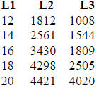
for male earnings
(12, 1812)
(14, 2561)
(16, 3430)
(18, 4298)
(20, 4421)
for female earnings
(12, 1008)
(14, 1544)
(16, 1809)
(18, 2505)
(20, 4020)
Put these values into lists L1, L2, and L3
Steps to use the TI -83 to plot the data
Press [Y=] and clear any function that is there. Then,
[STAT] [EDIT]
Enter corresponding values into L1, L2, and L3.
[2nd] [STATPLOT] [PLOT1] [on] Xlist: L1, Ylist: L2
[2nd] [STATPLOT] [PLOT2] [on] Xlist: L1, Ylist: L3
choose the second mark.
[Graph] to view the scatter plot. Adjust the window as necessary.
The two scatter plots will look as below. The lower, triangle points, represent
female
income.
Differences in earnings between male and female workers
are large. Women are earning
less than men at every educational level. Does this suggest labor-market
discrimination?
Not necessarily. Several factors can cause earnings disparities. Women may have
less
work experience than men, women may be less likely than men to work overtime or
to
choose occupations that offer jobs with high pay but long hours. Women may
choose
jobs closer to home than men. In addition, many women are concentrated in
occupations
that tend to pay lower wages. Even after taking into account these objective
factors, there
still remains a gap between the wages of males and females, that some attibute
to labor
market discrimination. In recent years, however, there has been a trend for this
gap to
decrease, especially for highly educated workers.
An inspection of the two graphs also suggests that there are different types of
lines that
best fit each of the data points. For males, a straight line seems acceptable,
but for
females the income points go up at an ever increasing rate. This suggests an
exponential
function (of the form  ) is a better fit than
a straight line.
) is a better fit than
a straight line.
To see this we will put the linear equation for the male incomes into equation
 , and
, and
the exponential regression equation for female incomes into equation

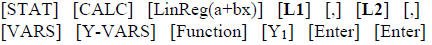
This puts the linear regression equation into the
![]() equation.
equation.

This puts the exponential equation into the
equation.
Press [Y=] to see the equations of the best fitting functions.
Males:

Females:
Now press graph to see these equations graphed through the points.
What do these graphs suggest regarding the importance of more education for
females as
compared with males? Does advanced education result in a proportionately larger
gain
for women than for men? How can this pattern be explained? Does this provide an
additional incentive for women to persue advanced degrees?
Additional Problems:
1. The male income points show an increase and then a decrease, this indicates
that
perhaps the male income can best be fit by a quadratic equation of the form

X2 + bX + c . Steps to use the TI-83 to graph a quadratic function.
Clear the existing  functions. Then enter:

a. What is the equation of the quadratic equation.
b. Which gives a better fit, the linear or the quadratic function?
c. If the quadratic fits better, what is its significance?
2. To be supplied.
3. Research: Use the Statistical Abstract of the United States to collect
data on
mean monthly income by highest degree earned according to race. Are any
differences in earnings between white and black workers? Graph the data and fit
a
straight line or exponential regression line to each data set. Can you give any
explanations for the differences in earnings between black and white workers
(other than discrimination)? There have been federal equal employment laws
against job discrimination based on race for over 30 years, as well as many
voluntary efforts to improve the employment of blacks and other minorities. If
these laws were effective, how would you expect them to affect the wage
differential between workers of different races?
| Prev | Next |