Methods For Interval Linear Equations
10. Using the inverse
Suppose we have a matrix P' which bounds the exact inverse P of A. In Section 4,
we
discussed how to obtain P'. Note that P'b bounds the hull h of the solution set.
The bound
on h would generally not be sharp even if P' were the exact inverse P. This is
because P can
contain matrices which are not inverses of any matrix in A. However, this
provides another
bound on h which can be intersected with bounds obtained by methods such as
those we
have described.
We can bound P more sharply than by the way described in Section 4 by using
methods
such as ours to solve the equations which P must satisfy. Thus, we can solve for
the ith
column of P by solving Ax =
![]() . We can solve for the
ith row of P by solving
. We can solve for the
ith row of P by solving  . If
. If
we solve for both the rows and the columns, we can intersect the two results .
The wider the vector b in Ax = b the wider the solution set. From this point of
view,
the equation Ax = ![]() is
ideal in that the right hand vector
is
ideal in that the right hand vector
![]() is real and all
components
is real and all
components
are zero except one. This suggests that there can be advantages in using a
method which
computes the inverse of A
11. Choosing a method
In practice, we must decide whether to use any of the methods we have described,
and,
if so, which one(s). We first note that if the center
![]() of A is "near" the
identity matrix,
of A is "near" the
identity matrix,
then its inverse B = ![]() is near the identity. In this case, there is little need to use any
is near the identity. In this case, there is little need to use any
of our methods. We can use B to precondition the system without unduly enlarging
the
solution set. We can then use the hull method to determine the hull of the
preconditioned
system. The question of what is meant by "near the identity matrix" will be left
to a user.
Alternatively, the center of A might be near a matrix which is the identity with
rows and
columns permuted.
Suppose the center ![]() of A is near the identity matrix. Then the center of A-1
is near
of A is near the identity matrix. Then the center of A-1
is near
the identity. That is, its off-diagonal elements are likely to contain zero.
Therefore, a row of
A-1 is unlikely to be SD. In this case, it is unlikely that our second method is
applicable,
and there is probably little point in using the fourth or sixth method.
For any problem, a reasonable first step is to obtain bounds xB on the hull h
using the
hull method. One can also use the method from [3] and find the intersection of
the two
methods Thereafter, we might use the following procedural steps. They involve a
great deal
of computing, but the work is polynomially bounded .
(1) If ![]() is near the (perhaps permuted) identity matrix, accept the results of
the hull
is near the (perhaps permuted) identity matrix, accept the results of
the hull
method as a sufficiently sharp solution. Thus, go to step (10).
(2) If xB is SD in all but a few components, solve for h using the first method
(in Section
3). Then go to step (10).
(3) Use the hull method to obtain bounds on A-1 by solving Ax =
![]() for i = 1,
..., n. (The
for i = 1,
..., n. (The
method in [3] can also be used.) Also solve
![]() for i = 1,..., n to bound
AT-1: Then
for i = 1,..., n to bound
AT-1: Then
intersect the two bounds on A-1: Denote the resulting bound on A-1 by PB.
(4) For i = 1, ., n, if all but a few components of row i of PB are SD, solve
for ![]() using the
using the
second method (in Section 4). If all components of h are obtained in this way,
go to step
(10).
(5) Compute the bound PBb on h: Intersect it with xB and the result from step
(4).
(6) If at least one component of h has been shown to be SD, the third method (in
Section
6) is applicable. Use it to bound h. Intersect the solution with the result of
step (5).
(7) Use the fourth method (in Section 7) to bound
 for i = 1, ..., n. Skip any
value of i for
for i = 1, ..., n. Skip any
value of i for
which was obtained sharply in step (4). Intersect the result with the result
from step (6).
(8) If at least one component of h has been found to be SD, use the fifth method
(in Section
8) to bound h. Intersect the result with the result from previous steps.
(9) Use the sixth method (in Section 9) to bound h. Intersect the result with
the result from
previous steps.
(10) Stop.
The amount of work to apply this procedure is not
particularly excessive if the crude
bounds reveal that h or A-1 is SD. If this is not the case, our procedure is
useful only if
sharpness is so important that a considerable amount of computing is warranted.
There are cases in which there is no need to use our methods. If A is an
M-matrix, then
interval Gaussian elimination will obtain the hull h sharply. See [5].
12. Some special cases
The essential requirement in our methods is that we are able to express certain
products in
which a factor is unknown except for its sign. For example, in the first method,
we needed
to be able to express Ax when x is unknown. If
![]() is SD, we can use (2.3) to
express
is SD, we can use (2.3) to
express 
in terms of the endpoints of  : But suppose that for a given value of j, the
element is
: But suppose that for a given value of j, the
element is
real (i.e., a degenerate interval) for all i = 1,..., n. Then the "endpoints"
of are equal,
and is expressed in terms of their coincident value. Therefore,
![]() need
not be SD.
need
not be SD.
If all but a few columns of A are real, the first method can be used to
determine the hull
h with a reasonable amount of computing. If a given column of A is real, the
corresponding
component of x does not have to be made SD in the third method, nor does it have
to be
eliminated in the fifth method.
Similar statements can be made for the dual methods. Now, however, we must be
able
to express both pTA and pT b for a row pT of P. Consider the matrix
 which
which
is the matrix P augmented with the vector b as an added column . If all but a few
rows of
R are real, the second method can determine the hull. If a row (or rows) of R is
real, the
corresponding component of a row of P need not be SD in the fourth and sixth
methods.
Even if every element of A except one is real, then every element of P can be a
nonde-
generate interval. It is unlikely that we shall know that a row of R is real.
Therefore, the
dual methods generally do not " simplify " in this way.
13. A non-polynomial method
The methods we have described fail if the crude methods fail to obtain bounds on
the
solution. In this section, we describe how the hull of the solution set of Ax =
b can be
obtained as the solution of an optimization problem. The optimization problem is
not
a linear programming problem, so the work to solve it is not polynomially
bounded. We
include it as an alternative for two reasons. First, it does not require that
some other method
provide crude bounds. Second, it is similar to the methods we have described.
The difference
is that the formulation of the optimization problem includes nonlinear
constraints.
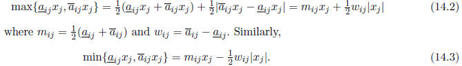
Equation (2.3) can be written as

Since the maximum of two function can be expressed as their average plus half
their difference,
we have
Row i of the equation Ax = b can be written
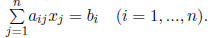
From (14.1), (14.2), and (14.3), we therefore obtain
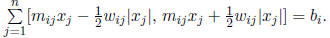
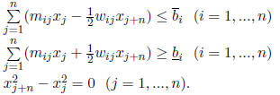
A point x is in the solution set of Ax = b only if the intervals in the left and right members
intersect. This imposes the constraints

and

for i = 1, ..., n.
We can obtain the kth component of the hull by minimizing and maximizing
 subject
to the constraints (14.4). The function  j is not differentiable at
![]() = 0. We
can obtain
= 0. We
can obtain
constraints which are differentiable if we replace
by  and add the
constraints
and add the
constraints
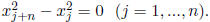
The problem now becomes: For k = 1, ..., n,
minimize and maximize
subject to
14. References
[1] Hansen, E. R., Interval arithmetic in matrix computations, part I, SIAM J.
Numer. Anal.
2, 308-320, 1965.
[2] Hansen, E. R., Global Optimization Using Interval Analysis, Marcel Dekker,
1992.
[3] Hansen, E. R., Sharpening interval computations, paper presented at the
First Scandi-
navian workshop on interval methods and their application, Copenhagen, 2003.
[4] Hansen, E. R. and Walster, G. W. Global Optimization
Using Interval Analysis, (second
ed.), Marcel Dekker, 2004.
[5] Heindl, G., Kreinovich, V., and Lakeyev, A. (1998), Solving linear interval
systems is
NP-hard even if we exclude overflow and underflow, Reliable Computing, 4, 383-388.
[6] Neumaier, A., Interval Methods for Systems of Equations, Cambridge
University Press,
London, 1990.
| Prev | Next |