Classification and Linear Equations

These notes cover some of the material that we covered in class on first-order ordinary
differential equations . As the presentation of this material in class was somewhat different
from that in the book, I felt that a written review closely following the class presentation
might be appreciated.

1. Introduction, Classification, and Overview

1.1. Introduction. A differential equation is an algebraic relation involving derivatives
of one or more unknown functions with respect to one or more independent variables, and
possibly either the unknown functions themselves or their independent variables, that hold
at each point in the domain of those functions.

For example, an unknown function p(t) might satisfy the relation

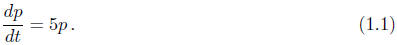
This is a differential equation because it involves the derivative of the unknown function
p. It also involves the value of p , but not the independent variable t. It is understood that
this relation should hold every point t where p(t) and its derivative are defined.

Similarly, unknown functions u(x, y) and v(x, y) might satisfy the relation

where and denote partial derivatives. This is a differential equation because it
involves derivatives of the unknown functions u and v. It does not involve either the values
of u and v or the independent variables x and y . It is understood that this relation should
hold every point (x, y) where u(x, y), v(x, y) and their partial derivatives appearing in (1.2)
are defined.

Here are other examples of differential equations that involve derivatives of a single
unkown function:

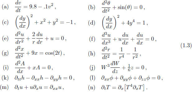
In all of these examples except k and l the unknown function itself also appears in the
equation. In examples d, e, g, i, and j the independent variable also appears in the equation.

1.2. Classification. A differential equation is called an ordinary differential equation
(ODE) if it invloves derivatives with respect to only one independent variable. Otherwise,
it is called a partial differential equation (PDE). Example (1.1) is an ordinary differential
equation. Example (1.2) is a partial differential equation. Of the examples in (1.3):

a – j are ordinary differential equations ;
k – n are partial differential equations .

The order of a differential equation is the order of the highest derivative that appears
in it. An n^th-order differential equation is one whose order is n. Examples (1.1) and (1.2)
are both first-order differential equations. Of the examples in (1.3):

a, c, d, j are first-order differential equations ;
b, e, g, h. i, k, l, m, n are second-order differential equations ;
f is a third-order differential equation .

A differential equation is said to be linear if each side of the equation is a sum of
terms, each of which either

• is a derivative of an unknown function times a factor that is independent of the
unknown functions,
• is an unknown function times a factor that is independent of the unknown fuctions,
• or is entirely independent of the unknown fuctions.

Otherwise it is said to be nonlinear. Examples (1.1) and (1.2) are both linear differential
equations. Of the examples in (1.3):

e, g, i, k, l are linear differential equations ;
a – d, f, h, j, m, n are nonlinear differential equations .

Every n^th order linear ordinary differential equation for a single unknown function y(t)
can be brought into the form

where , and r(t) are given functions of t such that p₀(t) ≠ 0. Linear
differential equations are important because much more can be said about them than for
general nonlinear differential equations.

In applications one is often faced with a system of coupled differential equations —
typically a system of m equations for m unknown functions. For example, two unknown
functions p(t) and q(t) might satisfy the system

Similarly, two unknown functions u(x, y) and v(x, y) might satisfy the system

The order of a system of differential equations is the order of the highest derivatrive
appearing in the entire system. Example (1.4) is a first-order system of ordinary differential
equations, while (1.5) is a first-order system of partial differential equations. The size of
the systems that arise in applications can be extremely large. Systems of 10⁸ ordinary
differential equations are being solved every day.

1.3. Course Overview. Differential equations arise in mathematics, physics, chem-
istry, biology, medicine, pharmacology, communications, electronics, finance, economics,
areospace, meteorology, climatology, oil recovery, hydrology, ecology, combustion, image
processing, and in many other fields. Partial differential equations are at the heart of most
of these applications. You need to know something about ordinary differential equations
before you study partial differential equations. This course will serve as your introduction
to ordinary differential equations. More specifically, we will study four classes of ordinary
differential equations. We illustrate these four classes below denoting the independent
variable by t.

(I) We will begin with single first-order ODEs that can be brought into the form

These will be covered before the first in-class exam. You may have seen some of the
material in your calculus courses.

(II) We will next study single n^th-order linear ODEs that can be brought into the form

These will be covered before the second in-class exam. This is the heart of the course.
Many students find this the most difficult part of the course.

(III) We will then turn towards systems of n first-order linear ODEs that can brought into
the form

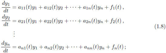
These will be covered before the third in-class exam. This material builds upon the
material covered in part II.

(IV) Finally, we will study systems of two first-order ODEs that can brought into the form

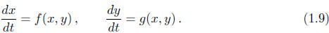
These will be covered before and immediately after the third in-class exam. This
material builds upon the material in parts I and III.

This is far from a complete treatment of the subject. It will however prepare you to learn
more about ordinary differential equations or to learn about partial differential equations.

2. First-Order Equations: Explict and Linear

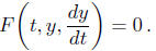
2.1. Introduction. We now begin our study of first-order ordinary differential equations
that involve a single real -valued unknown function y(t). These can always be brought into
the form

If we try to solve this equation for dy/dt in terms of t and y then there might be no solutions
or many solutions. For example, equation (c) of (1.3) clearly has no (real) solutions because
the sum of nonnegative terms cannot add to −1. On the other hand, equation (d) will be
satisfied if either

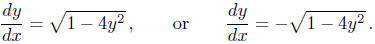
To avoid these complications we will restrict ourselves to equations that can be brought
into the form

Examples (1.1) and (a) of (1.3) are already in this form. Example (j) of (1.3) can easily
be brought into this form. And as we saw above, example (d) of (1.3) can be reduced to
two equations in this form.

We will say that y = Y (t) is a solution of (2.1) over an interval (a, b) whenever

Some basic questions we want to address are the following.

• When does (2.1) have solutions?
• Under what conditions is a solution unique?
• How can we find analytic expressions for solutions ?
• How can we visualize solutions?
• How can we approximate solutions?

We will focus on the last three questions. They address practical skills that you can apply
when faced with a differential equation. The first two questions will be viewed through
the lens of the last three. They are important because differential equations that arise in
applications are supposed to model or predict something. If an equation either does not
have solutions or has more than one solution then it fails to meet this objective. Moreover,
in those situations the methods by which we will address the last three questions can give
misleading results. We will therefore study the first two questions with an eye towards
avoiding such pitfalls. Rather than addressing these questions for a general f(t, y) in (2.1),
we will start by treating special forms f(t, y) of increasing complexity.