Least Squares and Curve Fitting
These notes cover a portion of the material in Chapter 5.4
of our text; my hope is that a somewhat less
thorough treatment may be easier to grasp. You may wish to fill in some of the
details by reading section
5.4.
The problem we will use for motivation is to find the
straight line that lies closest to a set of data points
in the plane. We will see that this leads directly to a question about solving
linear equations. To set this up,
consider a set of points (a1, b1), · · · (an, bn) in the plane. Maybe these
are measurements from an experiment;
for instance we might be measuring the movement of some particle, and the first
coordinate is time, while
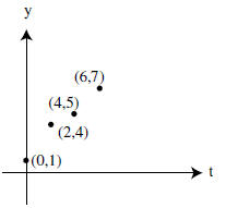
the second coordinate is position. We observe in the figures below, that the
data seem to lie near a line,
but not all on a line. We’d like to find an equation of a line that approximates
the data set, as drawn on
the left. To keep calculations to a minimum , we’ll work with the smaller data
set consisting of the points
(0, 1), (2, 4), (4, 5), (6, 7).
First, let’s observe why finding the straight line has anything to do with
solving linear equations. We
are looking for a line of the form
 that goes through all of the points. For each point
 , we
, we
must have
 which is a linear equation for the unknowns
 . So
if there were a line going
. So
if there were a line going
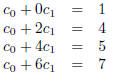
through all four points on the right- hand graph , the coefficients
 would
satisfy the system
would
satisfy the system
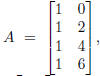
 or, in matrix form
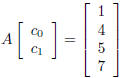 where
where

A quick reduction of A to rref shows that there is no solution to this system ,
which is pretty clear if you
examine the picture–the points just don’t lie on a line. In other terms , we can
say that the issue is that the
vector
 is not in the image of A.
This motivates the more general problem: given an m × n matrix A (giving a
linear transformation
 )
and a vector
)
and a vector
 ,
find the vector
,
find the vector
 that is closest to being a
solution to the equation
that is closest to being a
solution to the equation
 What do we mean by ‘closest to being a solution’? If
 is actually a
solution (ie
is actually a
solution (ie
 ) then that
would certainly qualify as closest. But, as in the curve fitting problem, there
may not be an actual solution.
The answer is provided by the following picture, in which we have written V =
Image(A).
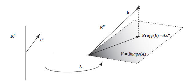
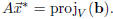
We are looking for the closest vector in V to b; the closest vector is given by
the projection of b into V .
This looks pretty clear in the picture; the book suggests a geometric proof on
pages 213-214. Since

lies in V = Image(A), we can write is as A times some vector. That vector is
 . So we have, in principle,
achieved our goal: we find our best approximation to a solution to
 by
solving (for
by
solving (for
 ) the equation
 We know that there is a solution, because the right hand side
is by definition an element
We know that there is a solution, because the right hand side
is by definition an element
of V . The vector
 is called a least -squares solution to the equation
 .
.
We can develop this a little further, and there are two reasons for doing so.
One is that projecting into
V is kind of a pain in the neck, since we’d have to find an orthogonal basis for
V in order to use our formula .
Also, it would be nice to have some kind of formula for
 . We’ll take care of
both of these at the same time.
. We’ll take care of
both of these at the same time.
(Obligatory disclaimer: in practice, especially with large systems, it’s often
better to just find the ON basis
for V and then solve for
 by Gaussian elimination. But fortunately we are not
worrying about such nasty
by Gaussian elimination. But fortunately we are not
worrying about such nasty
details!)
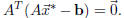
The main fact that leads us to a new solution is the one proved in Monday’s
class: a vector w is
perpendicular to V = Image(A) if and only if
 How does this help? Well,
to say that
How does this help? Well,
to say that

 is equivalent to saying that
 is perpendicular to V , which is
(by what we just observed)
is perpendicular to V , which is
(by what we just observed)
equivalent to
 The conclusion of all this is that
 is closest
to a solution of
is closest
to a solution of
 if and
only if it is a solution to the equation
The equation (that we solve to get
 ) is called the normal equation of
 . Note: we can solve this by
multiplying both sides by
 although in practice this may not be very
easy to compute.
although in practice this may not be very
easy to compute.
Let’s carry this out for the example we started with. We
have
 which gives

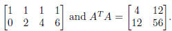 We also need
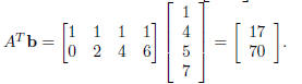
After some mildly messy arithmetic, we solve the system
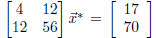 to get

Going back to the original problem, the line that best fits the data is given by
y = 1.4 + .95t. If there were
more data points, then the problem is pretty much the same, except that the
matrix A, which was 4 × 2 in
this example, will be k × 2 if there are k data points. If you like formulas,
you can find the general solution
to the normal equation at the end of chapter 5.4. You can also find another
worked example of how to find
a least-squares solution to an inconsistent equation in example 1 of section
5.4. In this example, the book
uses the fact that we can invert ATA to solve the normal equation.
There are some other variations on this theme. Suppose, for instance that a plot
of our data looks like a
parabola, suggesting that it might fit a quadratic equation. Thus, we would look
for a function of the form
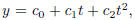 and so
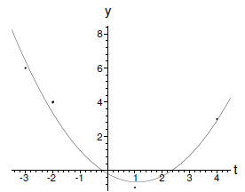
 has 3 variables. For example, the four data points below look like
they might fit a parabola.
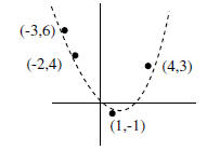
Plugging in the given values gives us equations
 etc. Thus we
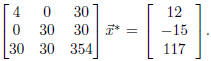
look for a good approximation to solutions to
 where
where
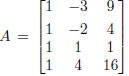 and
and
 As
As
above, we can’t solve the equation directly, so instead we solve the normal
equation
 This is
 After some work (I confess, I used a computer), I get
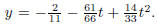
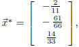 or
or
put another way, the best-fitting parabola is
 The corresponding parabola is drawn
below (again, done on the computer).
Homework problem 32 in this section leads to a more reasonable normal equation,
where you can do the
work by hand.
| Prev | Next |