Solving Systems of Linear Equations
Recall that we introduced the notion of matrices as a way of standardizing
the expression of systems of
linear equations . In today’s lecture I shall show how this matrix machinery can
also be used to solve such
systems. However, before we embark on solving systems of equations via matrices,
let me remind you of
what such solutions should look like.
1. The Geometry of Linear Systems
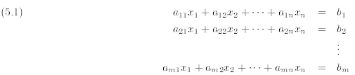
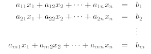
Consider a linear system of m equations and n unknowns:
What does the solution set look like? Let’s examine this question case by
case, in a setting where we can
easily visualize the solution sets.
• 0 equations in 3 unknowns. This would correspond to a situation where you
have 3 variables x 1, x2, x3
with no relations between them. Being free to choose whatever value we want for
each of the 3
variables, it’s clear that the solutions set is just R3, the 3-dimensional space
of ordered sets of 3 real
numbers .
• 1 equation in 3 unknowns. In this case, use the equation to express one
variable, say xn, in terms of
the other variables;
The remaining variables x1, and x2 are then unrestricted. Letting these
variables range freely over
R will then fill out a 2-dimensional plane in R2. Thus, in the case
of 1 equation in 3 unknowns we
have a two dimensional plane as a solution space.
• 2 equations in 2 unknowns. As in the preceding example , the solution set of
each individual equation
will be a 2-dimensional plane. The solution set of the pair of equation will be
the intersection of
these two planes. (For points common to both solution sets will be points
corresponding to the
solutions of both equations.) Here there will be three possibilities:
1. The two planes do not intersect. In other words, the two planes are
parallel but distinct.
Since they share no common point, there is no simultaneous solutoin of both
equations.
2. The intersection of the two planes is a line. This is the generic case.
3. The two planes coincide. In this case, the two equations must be somehow
redundant.
Thus we have either no solution, a 1-dimensional solution space (i.e. a line)
or a 2-dimensional
solution space.
• 3 equations and 3 unknowns. In this case, the solution set will correspond
to the intersection of the
three planes corresponding to the 3 equations. We will have four possiblities:
1. The three planes share no common point. In this case there will be no
solution.
2. The three planes have one point in common. This will be the generic
situation.
3. The three planes share a single line.
4. The three planes all coincide.
Thus, we either have no solution, a 0-dimensional solution (i.e., a point), a
1-dimensional solution
(i.e. a line) or a 2-dimensional solution.
We now summarize and generalize this discusion as follows.
Theorem 5.1. Consider a linear system of m equations and n unknowns:
The solution set of such a system is either:
1. The empty set {}; i.e., there is no solution.
2. A hyperplane of dimension greater than or equal to (n −m).
2. Elementary Row Operations
In the preceding lecture we remarked that our new-fangled matrix algebra
allowed us to represent linear
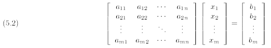
systems such as (5.1) succintly as matrix equations:
For example the linear system
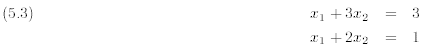
can be represented as
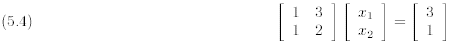
Now, when solving linear systems like (5.3) it is very common to create new,
but equivalent, equations by,
for example, mulitplying by a constant, or adding one equation to another. In
fact, we have
Theorem 5.2. Let S be a system of m linear equations in n unknowns and let S'
be another system of m
equations in n unknowns obtained from S by applying some combination of the
following operations:
• interchanging the order of two equations
• multiplying one equation by a non-zero constant
• replacing a equation with the sum of itself and a multiple of another equation
in the system.
Then the solution sets of S ane S' are identical.
In particular, the solution set of (5.3) is equivalent to solution set of
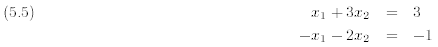
(where we have multiplied the second equation by -1), as well as the solution set of
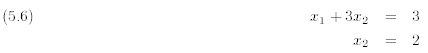
(where we have replaced the second row in (5.5) by its sum with the first row), as well as the solution of
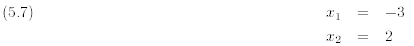
(where we have replaced the first row in (5.6) with its sum with −3 times the
second row). We can thus
solve a linear system by means of the elementary operations described in the
theorem above.
Now because there is a matrix equation corresponding to every system of
linear equations, each of the
operations described in the theorem above corresponds to an matrix operation. To
convert these operations
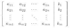
in our matrix language, we first associate with a linear system
an augmented matrix
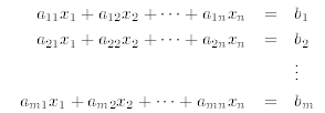
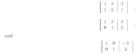
The augmented matrices corresponding to equations (5.5), (5.6), and (5.7) are thus, respectively
From this example, we can see that the operations in Theorem translate to the
following operations on the
corresponding augmented matrices:
• Row Interchange: the interchange of two row of the augmented matrix
• Row Scaling: multiplication of a row by a non-zero scalar
• Row Addition: replacing a row by its sum with s multiple of another row
Henceforth, we shall refer to these operations as Elementary Row Operations
3. Solving Linear Equations
Let’s now reverse directions and think about how to recognize when the system
of equations corresponding
to a given matrix is easily solved. (To keep our discussion simple , in the
examples given below we consider
systems of n equations in n unknowns.)
3.1. Diagonal Matrices. A matrix equation Ax = b is trivial to solve
if the matrix A is purely
diagonal. For then the augmented matrix has the form
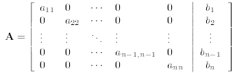
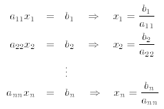
the corresponding system of equations reduces to
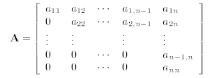
3.2. Lower Triangular Matrices. If the coefficient matrix A has the form
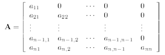
(with zeros everywhere above the diagonal from a11 to ann), then it is called
lower triangular. A matrix
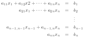
equation Ax = b in which A is lower triangular is also fairly easy to solve. For
it is equivalent ot a system
of equations of the form
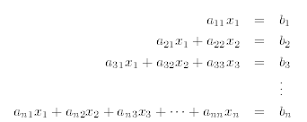
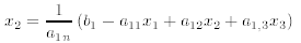
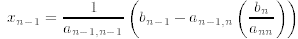
To find the solution of such a system one solves the first equation for x1
and then substitutes its solution
b1/a11 for the variable x1 in the second equation
One can now substitute the numerical expressions for x1, and x2 into the
third equation and get a numerical
expression for x3. Continuing in this manner we can solve the system completely.
We call this method
solution by forward substitution.
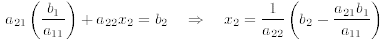
3.3. Upper Triangular Matrices. We can do a similar thing for systems
of equations characterized
by an upper triangular matrices A
(that is to say, a matrix with zero’s everywhere below and to the left of the
diagonal), then the corresponding
system of equations will be
which can be solved by substituting the solution of the last equation

into the preceding equation and solving for xn−1
and then substituting this result into the third from last
equation, etc. This method is called solution
by back-substitution.
3.4. Solution via Row Reduction. In the general
case a matrix will be neither be upper triangular or
lower triangular and so neither forward- or back-substituiton can be used to
solve the corresponding system
of equations. However, using the elementary row operations discussed in the
preceding section we can always
convert the augmented matrix of a (self-consistent) system of linear equations
into an equivalent matrix
that is upper triangular; and having done that we can then use back-substitution
to solve the corresponding
set of equations. We call this method Gaussian reduction. Let me
demonstate the Gaussian method with
an example.
Example 5.3. Solve the following system of equations using Gaussian reduction.
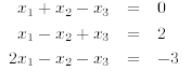
First we write down the corresponding augmented matrix.
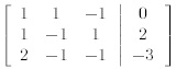
We now use elementary row operations to convert this
matrix into one that is upper triangular.
Adding -1 times the first row to the second row produces
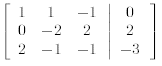
Adding -2 times the first row to the second row produces
Adding −3/2 times the second row to the third row produces
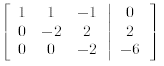
The augmented matrix is now in upper triangular form. It corresponds to the following system of equations
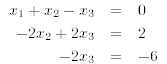
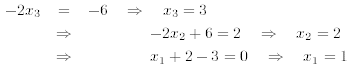
which can easily be solved via back-substitution:
In summary, solution by Gaussian reduction consists of the following steps
1. Write down the augmented matrix corresponding to the
system of linear equations to be solved.
2. Use elementary row operations to convert the augmented matrix into one that
is upper triangular.
This is acheived by systematically using the first row to eliminate the first
entries in the rows below
it, the second row to eliminate the second entries in the row below it, etc.
3. Once the augmented matrix has been reduced to upper triangular form, write
down the corresponding
set of linear equations and use back-substitution to complete the solution.
| Prev | Next |