Refresher on Probability and Matrix Operations

Outline

Matrix operations
Vectors and summation
Probability
Definitions
Calculating probabilities
Probability properties
Probability formulae
Random variables
Joint Probabilities
Definition
Independence
Conditional Probabilities

Matrix operations

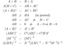
Here are some of the important properties of matrix and vector
operations. You don't need to memorize them, but you should
be able to apply them to questions on your problem sets.

What's different between the matrices A, B, and C versus L,
M, and N?

Since we are taking the inverses of the latter group , they must
be square and full rank. This is known as being non-singular.

Think of the matrix as a system of equations. each row in M is
a set of coefficients for the values of a vector of unknown
variables, say r, and solutions, s. If the matrix is invertible, you
can solve Ar = s.

In the context of regression, the M matrix is our observed
covariates (usually called X), s is a vector of outcomes (y), and
r is the vector of coefficients that we are trying to find ( β).

Vectors and summation

Define l as a conformable vector of ones.

We can express a sum in terms of vector multiplication:

We can do the same for a sum of squares of x:

Preliminary definitions

The sample space is the set of all possible outcomes of our
"experiment."

Note that experiment has the meaning in probability theory of
being any situation in which the final outcome is unknown and
is distinct from the way that we will define an experiment in
class.

An event is a collection of possible realizations from the
sample space.

Events are disjoint if they do not share a common element, i.e.,

An elementary event is an event that only contains a single
realization from the sample space.

Lastly, though getting a bit ahead, two events are statistically
independent if

Calculating probabilities

The classical definition of probability states that, for a sample
space containing equally- likely elementary events, then the
probability of an event is the ratio of the number of
elementary events in to that of , i.e.,

The axiomatic definition of probability defines probability by
stating that

for pairwise disjoint 1, : : : , n

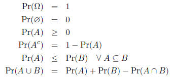
Probability properties

Let A and B be events in the sample space .

(Boole' s inequality )
(Bonferroni's inequality)

Probability formulae

The conditional probability of an event A given that an event B
has occurred is

This equation reflects that you received additional information
about the probability of A knowing that B occurred.

Pr(B) is in the denominator because the sample space has been
reduced from the full space to just that portion in which B
arises.

The law of total probability holds that, for a countable partition
of , and), then

Bayes' rule states that

for the two event case.

Random variables

A random variable is actually a function that maps every
outcome in the sample space to the real line . Formally,

If we want to find the probability of some subset of , we can
induce a probability onto a random variable X. Let X() = x.
Then,

Define the cumulative distribution function (CDF), , as
Pr(X≤ x). The CDF has three important properties:

(i.e., the CDF is non-decreasing)

A continuous random variable has a sample space with an
uncountable number of outcomes . Here, the CDF is defined as

For a discrete random variable, which has a countable number
of outcomes, the CDF is defined as

We can define the probability density function (PDF) for a
continuous variable as

by the Fundamental Theorem of Calculus.

It can be defined for a discrete random variable as

Note that

Joint Probabilities

Previously, we considered the distribution of a lone random
variable. Now we will consider the joint distribution of several
random variables. For simplicity , we will restrict ourselves to
the case of two random variables, but the provided results can
easily be extended to higher dimensions.

The joint cumulative distribution function (joint CDF),
, of the random variables X and Y is defined by

As with any CDF, must equal 1 as x and y go to
infinity.

The joint probability mass function (joint PMF), is defined
by

The joint probability density function (joint PDF), is
defined by

The marginal cumulative distribution function (marginal CDF)
of is

The marginal PMF of X is

The marginal PDF of X is

You are "integrating out" y from the joint PDF.

Note that, while a marginal PDF (PMF) can be found from a
joint PDF (PMF), the converse is not true, there are an infinite
number of joint PDFs (PMFs) that could be described by a
given marginal PDF (PMF).

Independence

If X and Y are independent, then

and

Conditional Probabilities

The conditional PDF (PMF) of Y given
is defined by

As for any PDF (PMF), over the support of Y , the conditional
PDF (PMF) must integrate (sum) to 1. It must also be
non- negative for all real values.

For discrete random variables, we see that the conditional PMF
is

Question: What is random in the conditional
distribution of Y ,

If X and Y are independent, then

This implies that knowing X gives you no additional ability to
predict Y , an intuitive notion underlying independence.