Introduction, Basics, Matlab
1.A Numerical Scheme
Consider the following example.
Example 1.1. Solve the quadratic equation

We can find the solution by performing some simple
algebraic manipulations leading to the
familiar quadratic formula:

Does this formula bring us any closer to finding the
numerical solutions of this problem? If we are
lucky, and b2−4c happens to be the square of some easily identifiable number, we
can compute the
solutions using a couple of additions and divisions . Likewise, almost any
calculator nowadays has a
built-in square root operation , and we can use it to find a numerical solution
even for general b and
c. Suppose however that we are able only to perform the four fundamental
arithmetic operations
of addition, subtraction, multiplication, and division. In this case, the
formula (2) is not much use,
unless we can somehow come up with a good numerical approximation to the square
root , obtained
using only +, −, ×, and /. Fortunately such schemes exist, as we discuss next.
1.1 Approximating the Square Root
So how do we calculate an approximate square root? Before we can answer, we must
consider two
of the fundamental limitations of numerical computation:
• Limited precision. Since there is only a limited amount of space to store any
number in
a computer , we cannot always store it exactly. Rather, we can only get a
solution that is
accurate up to the limit of our machine precision (for example, 16 digits of
accuracy ).
• Limited time. Each arithmetic operation (e.g. addition, multiplication) takes
time to perform.
Often we face a resource budget; the approximate solution must be available
within a limited
time.
Just to evaluate the quadratic function f(x) = ax2 + bx + c at a point x takes
time. Doing
it in the obvious way takes three multiplications (x * x, a * x2, b * x) and two
additions. (Q:
Can you see a faster way?)
We now present a method for funding the square root of a
given ( positive ) number c by generating
a sequence of guesses  , each of which is usually more accurate
than its predecessor.
, each of which is usually more accurate
than its predecessor.
 is the initial guess, which we supply;
 is the next guess obtained form our method;
 is the
one after that, and so on.
Our procedure uses the following simple formula to obtain each new guess
 from the previous
guess  :
:

If we start with an initial value
= 2.2 and carry out
this computation for three steps , we
obtain the following values of  , and
, and
 . (We also tabulate the squares of
these values, for
. (We also tabulate the squares of
these values, for
interest.)
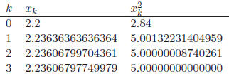
Using this procedure, only 3 × 4 = 12 simple arithmetic
operations are required to arrive at a
numerical solution that is accurate to the limit of Matlab’s precision. Taking
to be essentially
exact, and comparing it with the earlier values
 , and
, and
![]() , we see that
, we see that
![]() has 2 correct digits
has 2 correct digits
![]() has 4 correct digits,
and
has 4 correct digits,
and ![]() has 8 correct digits. The number of correct
digits doubles with each
has 8 correct digits. The number of correct
digits doubles with each
guess - a rapid rate of convergence.
Soon we will study the basis for the excellent performance of this scheme, which
is a particular
case of Newton’s method, and apply it to more complicated problems. In fact,
before going further,
we derive a generalization of this scheme for finding the roots of the quadratic
(1) directly, rather
than computing the square root approximation and plugging it into the formula
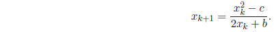
(2). Given one
approximation ![]() to a root of (1), we obtain the next guess by applying the
following formula:
to a root of (1), we obtain the next guess by applying the
following formula:

which, by simple elimination , is equivalent to the following:
2 Loss of Significance
Another issue in numerical computation is loss of significance. Consider two
real numbers stored
with 10 digits of precision beyond the decimal point :

If we subtract a from b , we will get the answer
0.0000000036. This result has only two significant
digits; it may differ from the underlying true value of this difference by more
than 1%. We have
lost most of the precision of the two original numbers.
One might try to solve this problem by increasing the
precision of the original numbers, but
this only improves the situation up to a point. Regardless of how high the
precision is, if it remains
finite, numbers that are close enough together will be indistinguishable. An
example of the effect
of loss of significance occurs in calculating derivatives.
Example 2.1 (Calculating Derivatives). Given the function f(t) = sint, what is f
'(2)?
We all know from calculus that the derivative of sin t is cos t, so one could
calculate cos(2) in
this case. However, just as with calculating definite integrals, it is not
always possible, or efficient
to evaluate the derivative of a function by hand.
| Tangent line to sin(2) | Secant line through sin(2), sin(2+h) |
 |
|
Figure 1: Tangent and Secant Lines on f(t) = sint
Instead, recall that the value of the derivative of a function f at a point  is the slope of the
line tangent to f at . Recall, also, that we can approximate this slope by
calculating the slope of
a secant line that intersects f at and at a point very close to , say
+h, as shown in Figure 2.
We learned in calculus, that as h → 0, the slope of the secant line approaches
the slope of the
tangent line, that is,

Just as with the definite integral, we could approximate
the derivative at by performing this
calculation for a small (but nonzero) value of h, and setting our approximate
derivative to be

This procedure is known as finite differencing. However,
notice that if h is very small, f(+h) and
f() are the same in finite precision. That is, the numerator of (6) will be
zero in finite precision,
and this calculation will erroneously report that all derivatives are zero.
Preventing loss of significance in our calculations will be an important part of
this course.
| Prev | Next |