Linear Systems of Equations

Outline

Preliminaries
Introductions.
Sign -up list.
Syllabus.
Homework 1.
Course Overview.
Linear Systems of Equations .

Key Points on Syllabus

Quizzes every Tuesday.
Homeworks due begining of class.
NO LATE HOMEWORKS.
Late projects are accepted with 20% penalty.
NO MAKEUP EXAMS. If you miss an exam, or if you do
badly, the weight of that exam will be added to the final .

Homework 1

Due Tuesday, Aug. 30, at beginning of class.

Section 1.1: 4,6,8,10,12,14,16,18,20, 23, 24, 30, 33,34
Section 1.2: 2,4,8,10,12, 15, 18, 20, 21,22, 24, 26, 29,
31, 33

Course Overview

Dealing with many variables and many equations.
Linearity.
Abstraction and Proofs.

Linear Equations

A linear equation in the variables is an equation
that can be written in the form

Examples:

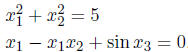
Not Linear:

Systems of Linear Equations

An m × n system of linear equations has the form:

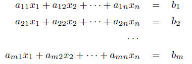
Note: each equation involves the same variables, .
A solution of the system is a list of numbers () that makes each equation
true when the values are substituted for , respectively.

Example: The system

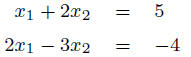
has solution .

A Geometric View

Exercises:

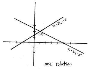
Graph the solution set of the equation . (Question: why does it make
sense to call this a linear equation?).

Graph the line defined by the equation .

Where do these two lines intersect?

Geometry 2

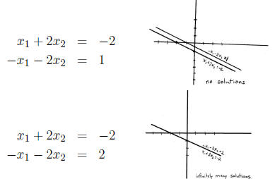
But this doesn’t always work:

Solutions of Linear Systems

A system of linear equations has either
1. No solution (inconsistent).
2. Exactly one solution. (consistent).
3. Infinitely many solutions. (also consistent).

Matrix Notation

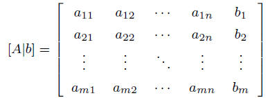
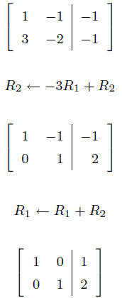
Since all the equations in a linear system involve the same variables, we can economize by
writing only the coefficients (not the variables) in a compact form called the Augmented
matrix:

Example:

Solving Linear Systems

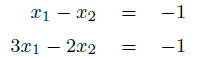
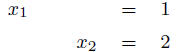
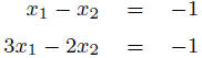
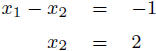
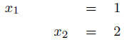
Add (-3) times equation 1 to equation
2.

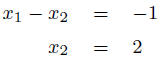
Add equation 2 to equation 1.

Add (-3) times equation 1 to equation 2.
Add equation 2 to equation 1.

Elementary Row Operations

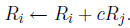
1. (Replacement) Add c times row j to row i (replacing row
i, and leaving row j unchanged).

2. (Interchange) Interchange row i and row j.



3. (Scaling) Multiply row i by a constant c ≠ 0.



KEY FACT: Elementary row operations do not alter the
solution set.

Gauss- Jordan Elimination

Apply a sequence of elementary row operations to get the matrix into a form that is
trivial to solve.

Example: A series of elementary row operations yields the following transformation

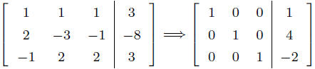
The righthand matrix corresponds to the system of equations:

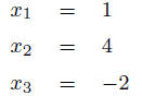
Trivial to solve!!
The above matrix is in a special form called the reduced row echelon form.