Finding Complex Zeros of a Quadratic Function Grap

Identifying Quadratic Functions; Concavity

We can recognize a quadratic function algebraically by that fact that the formula for the function can only contain three types of terms: constant terms, and variable terms where the independent variable is to the first or second power. Graphically, of course, we recognize a quadratic function as a parabola. How can we identify a quadratic function numerically; that is, from a table of data? With a linear function , we look for a constant rate of change. With a quadratic function, it turns out that the rate of change of the rate of change is constant.

Consider the function f(x) = −16x² + 40x + 5 Table 1 shows some values for f using a uniform change in x of Δx = 0.2.

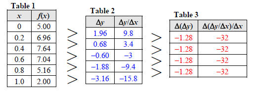
In Table 2 we have calculated the differences in y, Δy, as well as the average rate of change in f with respect to x, Δy/Δx, between consecutive pairs of points. For example, on the interval [0, 0.2], we have

Note: With calculus it can be shown that, for a
quadratic function, the instantaneous rate of change
in y with respect to x is a linear function of x.

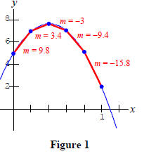
We see that the average rates of change, Δy/Δx, are decreasing. Graphically, this means that the slopes of the secant lines are decreasing (going from positive to negative ) as illustrated in Figure 1. More importantly, notice that the values of Δy and Δy/Δx are decreasing at a steady rate (the values in the Table 2 form arithmetic sequences).

Table 3 shows the second differences, Δ(Δy), and average rate of change in Δy/Δx with respect to x, or Δ(Δy/Δx)/Δx. For instance, using the values in the first two rows of Table 2 we have

Because the values in Table 2 are decreasing at a steady rate, the values in Table 3 remain
constant. Thus, with a quadratic function, whenever there is a uniform increment Δx the
second differences in y will be constant. In addition, the rate of change of the rate of change
is constant as well. This leads us to the following property.

PROPERTY OF QUADRATIC FUNCTIONS

For a quadratic function, the rate of change of the rate of change is a constant.

The average rate of change of the average rate of change can also be expressed as

For example, using the first two values in the first column of Table 2 gives us

EXAMPLE 1 Identifying a Quadratic Function from a Table

Determine which of the following functions could be quadratic.

SOLUTION

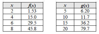
Both tables have a uniform Δx. We check the data for each function to see if the second differences in y are constant. For f, we see that the second differences do not appear to be constant, so this function is not quadratic.

The second differences for g seem to be constant, so this function could be quadratic.

To compute the average rate of change of the average rate of change, we can simply divide Δ(Δy) by (Δx)², resulting in
19/(52) = 0.76.

CONCAVITY

In Figure 1 we can see that, because the rate of change is not constant, the graph is forced to bend or curve . The rate at which
the slopes Δy/Δx are increasing or decreasing gives us some idea of how rapidly the graph of the function is curving, or
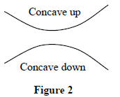
bending, and the sign of this rate indicates the direction in which the graph is curving. If Δ(Δy)/(Δx)² is positive, then the rate of change in f is increasing with x and the graph will bend in an upward direction (like a spoon held
right-side up) as illustrated in Figure 2. We say the graph is concave up. If Δ(Δy)/(Δx)² is negative,
then the rate of change in f is decreasing with x and the graph will bend in a downward direction
( like a spoon held upside-down). We say the graph is concave down. For example, with
f(x) = −16x² + 40x + 5, we saw that Δ(Δy)/(Δx)² = −32 so the graph will be concave down as Figure
1 indicates.

Since Δ(Δy)/(Δx)² for a quadratic function is constant, the concavity of its graph (a parabola)
will never change. That is, the graph will either be concave up or concave down over the entire
domain. In Exercise 00 it is shown that

so that the concavity is determined by the sign of the leading coefficient , a. This is consistent with the observations we made earlier in this section about whether the parabola opens upward or opens downward based on the sign of a.

CONCAVITY OF QUADRATIC FUNCTIONS

The graph of the quadratic function f(x) = ax² + bx + c will be concave up if a > 0 and concave down if a < 0.

EXAMPLE 2 Determining the Concavity of a Quadratic Function

Determine the concavity of the graph of g(x) from Example 1.

SOLUTION

To compute the average rate of change of the average rate of change in g, we can simply divide Δ(Δy) by (Δx)², resulting in 19/(25) = 0.76. This rate is positive, so the graph of g is concave up over its entire domain. Since 2a = 0.76, we also know that the coefficient of the x2 term for g must be equal to 0.38.

EXERISES

Determine whether the graph of each function is concave up or concave down.

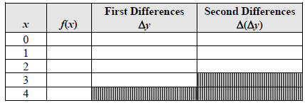
3. Use the function f (x) = x² +11x − 9 to complete the table below.

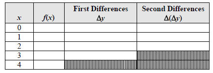
4. Use the function f (x) = −3x² + x + 5 to complete the table below.

For Exercises 5-6, show that the given data is indicative of a quadratic function and determine the concavity. For Exercises 7-8, determine whether the function could be quadratic. Explain your reasoning

9. Sketch a possible graph for a function f under each set of circumstances.
(a) f is increasing and concave up
(b) f is increasing and concave down
(c) f is decreasing and concave up
(d) f is decreasing and concave down

10. Roller Coasters The function d = f(t) gives the distance d, in feet, traveled by a rollercoaster after t seconds. Data for the first three seconds is shown in the following table.

(a) Find the average rate of change in f with respect to t on the interval [1, 2]. What does this value represent in
practical terms ?
(b) Find the average rate of change in f with respect to t on the interval [2, 3].
(c) Acceleration is the rate of change in velocity over time. Assuming the acceleration is constant, use your answers
from (a) and (b) to find the acceleration of the rollercoaster. Include units with your answer.