Inverse Trigonometric Functions
In this section we will introduce the inverse
trigonometric functions . We will begin with
the inverse tangent function since, as indicated in Section 6.4, we need it to
complete the
story of the integration of rational functions .
Strictly speaking, the tangent function does not have an inverse. Recall that in
order
for a function f to have an inverse function, for every y in the range of f
there must be
exactly one x in the domain of f such that f(x) = y. This is false for the
tangent function
since, for example, both tan(0) = 0 and tan(π ) = 0. In fact, since the
tangent function is
periodic with period π, if tan(x) = y, then tan(x + nπ ) = y for any
integer n. However,
the tangent function is increasing on the interval
 , taking on every value in its
range (−∞,∞) exactly once. Hence we may define an inverse for the tangent
function
if we consider it with the restricted domain .
That is, we will define an inverse
tangent function so that it takes on only values in
.
Definition The arc tangent function, with value at x denoted by either
arctan(x) or
tan-1(x), is the inverse of the tangent function with restricted domain
.
In other words, for  ,
,
y = tan-1(x) if and only if tan(y) = x.
 (6.5.1)
For example,  , and
, and
 . In particular, note that
even though  since 0 is between
 and
and  , but
π is not between
, but
π is not between
and .
The domain of the arc tangent function is (−∞,∞), the range of the tangent
function,
and the range of the arc tangent function is ,
the domain of the restricted tangent
function. Moreover, since

and

we have

and

Figure 6.5.1 Graph of y = tan-1(x)
Hence  and
and  are horizontal asymptotes for the graph of y = tan-1(x), as
shown in Figure 6.5.1.
To differentiate the arc tangent function we imitate the method we used to
differentiate
the logarithm function . Namely, if y = tan-1(x), then tan(y) = x, so
Hence

from which it follows that
Now

so we have
Hence we have demonstrated the following proposition.
Proposition

As a consequence of the proposition, we also have

Note that 1+x2 is an irreducible quadratic polynomial. We
will see more examples of
this type in the following examples.
Example Using the chain rule, we have
Example Evaluating  is
similar to evaluating
is
similar to evaluating  . That is, we will
use integration by parts with
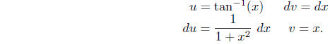
Then

Using the substitution
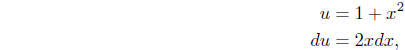
we have  , from which it
follows that
, from which it
follows that

Thus

Example To evaluate 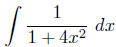 ,
we make the substitution
,
we make the substitution
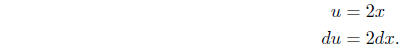
Then  , so
, so

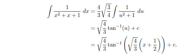
Example To evaluate 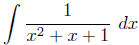 ,
we first note that x2 + x + 1 does not factor,
,
we first note that x2 + x + 1 does not factor,
that is, is irreducible, and so we cannot use a partial fraction decomposition .
In general,
a quadratic polynomial ax 2 + bx + c is irreducible if b2 −
4ac < 0 since, in that case, the
quadratic formula yields complex solutions for the equation ax2+bx+c = 0. For
x2+x+1
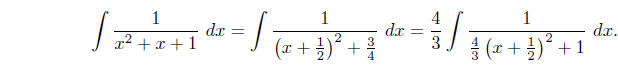
we have b2 − 4ac = −3. In this case it is helpful to simplify the function
algebraically by
completing the square of the denominator , thus making the problem similar to the
previous
example. That is, since

we have
Now we can make the substitution
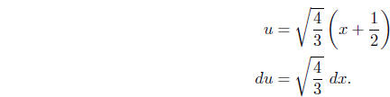
Then 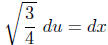 , so
, so
Partial fraction decomposition: Irreducible quadratic
factors
The last two examples illustrate techniques that we may use to evaluate the
integral of
a rational function with an irreducible quadratic polynomial in the denominator.
With
this we are now in a position to consider the final case of partial fraction
decomposition.
Specifically, suppose we want to evaluate
where f and g are both polynomials and the degree of f is
less than the degree of g.
Moreover, suppose that (ax2 + bx + c)n is a factor of g, where n is a positive
integer and
ax2 + bx + c is irreducible. Then the partial fraction
decomposition of  must contain
a sum of terms of the form

where  and
and
 are constants. Note that the terms in the
partial
are constants. Note that the terms in the
partial
fraction decomposition corresponding to an irreducible quadratic factor differ
from the
terms for a linear factor in that the numerators of the terms in (6.5.6) need
not be constants,
but may be first degree polynomials themselves. As before, this is best
illustrated with an
example.
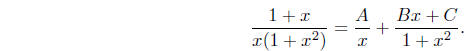
Example To evaluate  we need to find
constants A, B, and C such that
we need to find
constants A, B, and C such that
Combining the terms on the right, we have

Hence

Equating the coefficients of the polynomials on the left
and right gives us the system of
equations
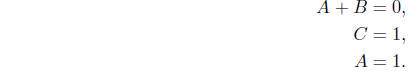
Thus B = −1 and

Hence
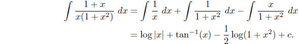
where the final integral follows from the substitution u =
1 + x2 as in an earlier example.
If, unlike this example , the partial fraction decomposition of
![]() results in a term of
results in a term of
the form
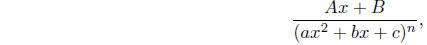
where n > 1 and ax2 + bx + c is irreducible,
then the integration may still be difficult to
carry out, perhaps even requiring some of the ideas of trigonometric
substitutions that we
will discuss in the next section. However, there is a limit to what should be
done without
the aid of a computer, or at least a table of integrals. There is a point after
which some
integrations become so complicated and time-consuming that in practice they
should be
given to a computer algebra system .
| Prev | Next |