Solving Linear Equations
18.1 Introduction
This lecture is about solving linear equations of the form Ax = b, where A is
a symmetric positive
semi-definite matrix. In fact, we will usually assume that A is diagonally
dominant, and will
sometimes assume that it is in fact positive definite .
We will brie y describe the Chebyshev method for solving such systems, and
the related Conjugate
Gradient. We will then explain how these methods can be accelerated by
preconditioning. In
the next few lectures, we will see how material from the class can be applied to
construct good
preconditioners.
18.2 Approximate Inverses
In undergraduate linear algebra classes , we are taught to solve a system like
Ax = b by first
computing the inverse of A, call it C, and then setting x = Cb. However, this
can take way too
long. In this lecture, we will see some ways of quickly computing approximate
inverses of A, when A
is symmetric and positive semi-definite. By "quickly", we mean that we might not
actually compute
the entries of the approximate inverse, but rather just provide a fast procedure
for multiplying it
by a vector. I'll talk more about that part later, so let's first consider a
reasonable notion of
approximate.
The fact that the inverse C satisfies AC = I is equivalent to saying that all
eigenvalues of AC are
1. We will call C an -approximate inverse of A if all eigenvalues of AC lie in
 In
In
this case, all eigenvalues of I - AC lie in
 from which we can see that C can be used to
approximately solve linear systems in A. If we set x = Cb, then
In our construction, we will guarantee that AC is symmetric, and so
 and
and

18.3 Chebyshev Polynomials
We will exploit matrices C of the form

Note that one can quickly compute the product Cb : we will iteratiely compute
Aib, and then take
the sum . So, if A has m non- zero entries , then this will take O(mt) steps. I
should warn you that
I'm ignoring some numerical issues here.
Now, let's find a good choice of polynomials. Recall that we want

to have all its eigenvalues between
 .
Let
.
Let
Then, for each eigenvalue
 is an eigenvalue of I - AC. Assuming that A is positive
definite, its eigenvalues all lie between
 and
and
 where
where
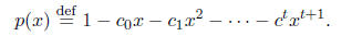
 So, it suffices to find a
polynomial p with constant term 1 such that
 for all
 As in Lecture 8,
we will use Chebyshev polynomials to construct p. We recall that the k-th
Chebyshev polynomial,
Tk, has the following properties
1.
Tk has degree k.
2.
3.
Tk(x) is monotonically increasing for x≥1.
4.

To express p(x) in terms of a Chebyshev polynomial, we should map the range
on which we want
p to be small,
 to [-1, 1]. We will accomplish this with the linear map:
Note that
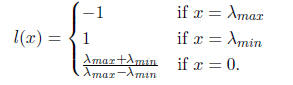
So, to guarantee that the constant coefficient in p(x) is zero, we should set
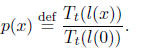
We know that
 To find p(x) for x in this range, we must compute
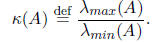
 We will express the result of our computation in terms of the condition number
of , which
We will express the result of our computation in terms of the condition number
of , which
for a symmetric matrix is
We have
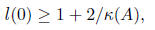
and so by properties 3 and 4 of Chebyshev polynomials,
Thus,
for
 and so all eigenvalues of I-AC will have absolute value at most
So, to get accuracy
 in our solution to Ax = b, we need
18.4 Computational properties, and the Conjugate Gradient
The Chebyshev properties have some useful properties that I should mention,
but which I will not
prove. The most useful property is that their coefficients have a clean
recursive definition. As a
result, we can construct an algorithm, called the Chebyshev method, that just
takes as input a
lower bound on
 and an upper bound on
 and, after t iterations produces the estimate
obtained from
 .
In particular, the algorithm is iterative, and at each iteration obtain the
correct
.
In particular, the algorithm is iterative, and at each iteration obtain the
correct
estimate.
The Chebyshev method is not used much in practice because there is a better
method|the Conjugate
Gradient. The CG method adaptively computes the coefficients of the polynomial,
and is
guaranteed to compute the optimal coefficients at each iteration. I will now dwell
on how it works
now, but I will mention that it is quite efficient, and always at least as good as
the Chebyshev
method.
18.5 Preconditioning
So, we know that we can obtain an approximate solution to a system of the
form Ax = b in time
depending on
 But, what if
 is large? In this case, we can try to precondition A .
That means finding a matrix B that is similar to A, but for which it is easy to
solve equations like
Bz = c. We then apply the Chebyshev method, or the Conjugate Gradient, to solve
The running time of the preconditioned method is effected in two ways :
1. At each iteration, in addition to multiplying a vector by A, we must solve
a linear system
Bz = c, which we can think of as multiplying by B-1, and
2. The number of iterations now depends the eigenvalues of
(B-1A). If A and B are positive
definite, then all the eigenvalues of B-1A will be real and non-negative, so the
number of
iterations just depends upon

Note that I am ignoring one detail that B-1A is not
symmetric. Please just trust me for now that
this doesn't make much difference, so I can get through the rest of the lecture.
Our goal in preconditioning is to find a matrix B that
guarantees that the eigenvalues of B-1A are
not too big, and so that it is easy to solve a linear system in B. It will help
if I give a different
characterization of 
| Prev | Next |