Linear Homogeneous Second- Order Ordinary Differential Equations Analysis and Visualization

Example  10.6
Show that for all real numbers and

is a solution to the ODE

Solution: Calculate

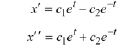
Then

hence is a solution to the ODE.

End of Example 10.6

The last example admits the following generalization.

Theorem 10.7 [Linearity]
If and are solutions to Eqn. (10.4)

then for all real numbers and the linear combination

is also a solution.

Definition 10.8 [Characteristic Polynomial]
The polynomial

is called the characteristic polynomial for the homogeneous ODE

The roots of the characteristic polynomial are called its characteristic roots.

The characteristic roots can be classified into one of three categories:
• Real distinct; i.e.
• Real identical; i.e.,
• Complex conjugate ; i.e., with

For instance. if and are real distinct, we see that

must be solutions to Eqn. (10.4). Even when the roots and are identical or are complex conjugate, we will determine
appropriate solutions. The next theorem provides these.

Theorem 10.9 [General Solution]
Suppose the coefficients and are real numbers and that the characteristic polynomial has roots
and There are three possibilities for a general solution to

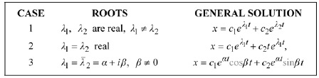
where and are arbitrary real numbers. Each of these solutions is defined at for all

Proof:

Observe that we can set and or and in Example 10.6 to obtain the particular solutions and
In fact, we can do the same in Case 1 of Theorem 10.9 to get the particular solutions and These
particular solutions will play an important role in the theory of linear second -order ODEs with constant coefficients .

Example 10.10:
Determine the general solution to the ODE

Solution: The characteristic equation is As this polynomial doesn't factor readily , use the quadratic formula to calculate the
characteristic roots

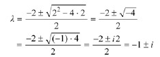
to get complex conjugate roots Note that So according to Theorem 10.6, Case 3 prevails so that the general solution is

The reader should check this;, i.e., verify that is a solution to the ODE.
End of Example 10.10

Observe that we can set in Example 10.9 to obtain the particular solutions
and In fact, we can do the same in Case 3 of Theorem 10.9 to get the particular solutions and
In fact, the particular solutions obtained by setting in Theorem 10.6 are
distinguished by the role they play with regard solving an IVP for

Theorem 10.6 begs the question: Do these cases cover all possible solutions? Given a set of initial conditions, say
can we be confident that one of the three cases provides a unique solution? The answer is YES as we shall soon
see. But first we examine how initial values affect solutions.

10.4 INITIAL CONDITIONS

Whereas a first-order ODE generally admits a single solution that satisfies a second-order ODE can
have infinitely many solutions satisfying It is instructive to examine a simple ODE and see why this is so.
Consider the ODE

Calculate the characteristic roots by solving the quadratic equation

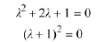
Thus we get the real repeated root

From Case 2 of Theorem 10.9, the general solution is

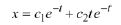
Now suppose we wish to determine the solution that satisfies Thus we must have

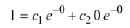
which implies

As no restriction is placed on we can only say that the solution is

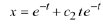
Consequently, there are infinitely many solutions - one for each value of Figure 10.5(a) depicts four such solutions.

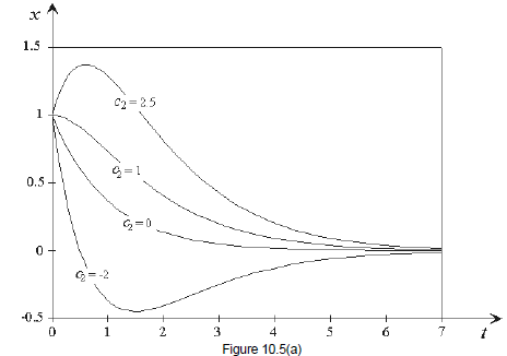
Observe how each of the solutions issues forth from the initial point Each solution has a different slope at We
can calculate these from the corresponding solutions. Since then

For each value of we calculate the corresponding value of the slope of the corresponding solution at For
instance, when

The following table lists these values.

Figure 10.5(b) displays the same graphs , this time labeled with the values of instead of

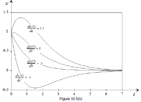
We see from the preceding analysis of the solutions to that specification of a value for and a value for
is sufficient to uniquely determine a solution. With this in mind we can define what we mean by initial conditions and
an IVP for a linear homogeneous second-order ODE.

Definition 10.11 (Initial Value Problem)

An initial value problem (IVP) for a linear homogeneous second-order ODE consists of two things :
1. An ODE

and

2. Initial Conditions

where are given numbers and are called initial values or initial data.