Introduction to R Workshop
1 Introduction
In this lab, we will be exploring how to use R. We will
work on generating and accessing
elements/components from R objects including vectors, matrices, lists, factors ,
data frames
and functions (both built in and user defined). We will also explore R's basic
graphics utilities
including plot, hist, and boxplot. Finally, we'll introduce you to R's control
structures:
if-else, for and while loops. Have fun!
2 Vectors
Create a numerical vector of all the integers from 11 to
20 named num using the sequence
generating operator :. Use this vector to generate 6 logical vectors named
lg1...lg6 by
applying conditions using comparison operators >, >=, <, <=, == and !=. Generate
a character
vector named char using the concatenate function c(...). Use this vector to
create 2 logical
vectors, lg7 and lg8, using the comparison operators == and !=. View the
elements of all
these vectors by typing their names and hitting "enter" on your keyboard. Create
a mixed
vector named mix1 that contains values with a decimal point and integers using
the c(...)
function. What type of vector is produced? Check by typing mix1 and hitting
"enter" on
your keyboard as well as using the mode(...) function. Create a mixed vector
named mix2
that contains values with a decimal point , integers and characters with the
c(...) function.
What type of vector is produced? Again, check by typing mix2 and hitting "enter"
on your
keyboard as well as using the mode function.
Extract a subset of elements from num using the :
operator, c(...) as well as all 6 of
the logical vectors lg1...lg6. Extract the elements of char by using lg7 and
lg8. Extract
subsets of mix1 and mix2 using negative indexes together with the : operator and
the c(...)
function.
Perform the following mathematical operations on num :
num/num, num*num, num**2, num
+ num, 2*num and num - num. Are these standard matrix operations?
> num = 11:20
> num # components of num
[1] 11 12 13 14 15 16 17 18 19 20
> lg1 = num > 15
> lg1 # components of lg1
[1] FALSE FALSE FALSE FALSE FALSE TRUE TRUE TRUE TRUE TRUE
> lg2 = num < 12
> lg3 = num >= 16
> lg4 = num <= 10
> lg5 = num == 20
> lg6 = num != 11
> char = c("R", "Perl", "stats", "bioconductor", "ChIP-Seq")
> lg7 = char == "R"
> lg8 = char != "Perl"
> mix1 = c(1, 2, 3.3)
> mix1 # doubles
[1] 1.0 2.0 3.3
> mode(mix1)
[1] "numeric"
> mix2 = c(1, 2, 3.3, "R")
> mix2 # character
[1] "1" "2" "3.3" "R"
> mode(mix2)
[1] "character"
> num[2:6]
[1] 12 13 14 15 16
> num[c(1,3,5)]
[1] 11 13 15
> num[lg1]
[1] 16 17 18 19 20
> num[lg2]
[1] 11
> num[lg3]
[1] 16 17 18 19 20
> num[lg4]
integer(0)
> num[lg5]
[1] 20
> num[lg6]
[1] 12 13 14 15 16 17 18 19 20
> char[lg7]
[1] "R"
> char[lg8]
[1] "R" "stats" "bioconductor" "ChIP-Seq"
> mix1[-(3:4)]
[1] 1 2
> mix2[-c(3,4)]
[1] "1" "2"
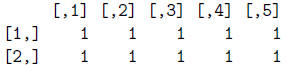
> num/num
[1] 1 1 1 1 1 1 1 1 1 1
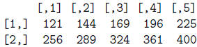
> num*num
[1] 121 144 169 196 225 256 289 324 361 400
> num**2
[1] 121 144 169 196 225 256 289 324 361 400
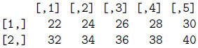
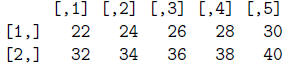
> num+num
[1] 22 24 26 28 30 32 34 36 38 40
> 2*num
[1] 22 24 26 28 30 32 34 36 38 40
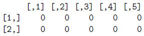
> num-num
[1] 0 0 0 0 0 0 0 0 0 0
3 Matrices
Create a 5 column matrix named mat from num using the
matrix() function and lling in
the values by row first. What are the dimensions of mat? Type mat at the prompt
then
"enter" and use the dim() function to find out. Extract the element in the second
row and
third column of mat. Extract the full first row and, separately, the full fourth
column of
mat. Extract all rows and the 4th and 5th columns of mat using the : operator
and c()
command. Create a logical vector lg9 by checking to see which elements in the
rst row
of mat are <= 14. Apply lg9 to the columns of mat. Perform the following
mathematical
operations on mat: mat/mat, mat*mat, mat**2, mat + mat, 2*mat and mat - mat.
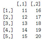
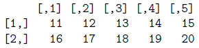
> mat = matrix(num, ncol=5, byrow=T)
> mat
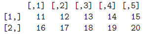
> dim(mat)
[1] 2 5
> mat[2,3]
[1] 18
> mat[1,]
[1] 11 12 13 14 15
> mat[,4]
[1] 14 19
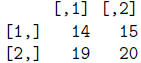
> mat[,4:5]
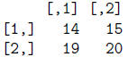
> mat[,c(4,5)]
> lg9 = mat[1,] <= 14
> lg9
[1] TRUE TRUE TRUE TRUE FALSE
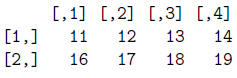
> mat[,lg9]
> mat/mat
> mat*mat
> mat**2
> mat + mat
> 2*mat
 > mat-mat
4 Lists and Data Frames
Generate a list named ExpList with three components:
ExpLevel (3 numeric elements),
Exp (3 logical elements with at least one TRUE ) and GeneName (3 character
elements). Type
ExpList and hit "enter". Extract the GeneName component using the $ operator,
double
brackets,[[]], and single brackets, [], after ExpList. Do you notice any di
erences in the
outputs? Extract the third element of the GeneName component. Extract the
ExpLevel
and GeneName components in one view using single brackets after ExpList, [].
Generate a
character vector of length 3 named ids. Type help(as.data.frame). Read the help
page.
Apply the function as.data.frame on the list ExpList to generate a data frame
named
ExpData with row names ids (setting stringsAsFactors=F). Type ExpData and hit
"enter".
Extract the rst row and then the third column ( two separate operations) of
ExpData using
indexes. Use the $ operator to extract the Exp column. Extract the rows that are
TRUE
in the Exp column. Check the attributes of ExpData by applying the dim() and
mode()
functions.
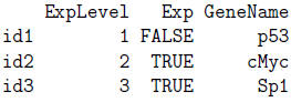
> ExpList = list(ExpLevel=c(1,2,3), Exp=c(F,T,T), GeneName=c("p53",
"cMyc", "Sp1"))
> ExpList
$ExpLevel
[1] 1 2 3
$Exp
[1] FALSE TRUE TRUE
$GeneName
[1] "p53" "cMyc" "Sp1"
> ExpList$GeneName
[1] "p53" "cMyc" "Sp1"
> ExpList[[2]]
[1] FALSE TRUE TRUE
> ExpList[2]
$Exp
[1] FALSE TRUE TRUE
> ExpList$GeneName[3]
[1] "Sp1"
> ExpList[c(1,3)]
$ExpLevel
[1] 1 2 3
$GeneName
[1] "p53" "cMyc" "Sp1"
> ids = c("id1", "id2", "id3")
> ExpData = as.data.frame(ExpList, row.names=ids, stringsAsFactors=F)
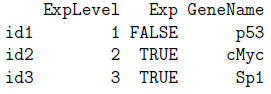
> ExpData
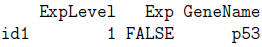
> ExpData[1,]
> ExpData[,3]
[1] "p53" "cMyc" "Sp1"
> ExpData$Exp
[1] FALSE TRUE TRUE
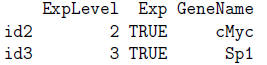
> ExpData[ExpData$Exp,]
> dim(ExpData)
[1] 3 3
> mode(ExpData)
[1] "list"
5 Reading and Writing Data
Now we're going to learn to read and write data into and
out of R respectively. We're going
to start by writing so that we have les to read in. First, we're going to write
the matrix mat
to a le named "mat.txt". We'll use the write() function which writes a vector or
matrix
to a le. Type help(write). You'll see that write requires you to transpose your
matrix
(i.e., switch rows and columns). So try the following:
> t(mat) #transpose mat matrix
> write(t(mat), file="matrix.txt", ncol=5, sep="\t")
Check to see if the le"matrix.txt"is in the same directory
in which you called R by typing
system("ls"). If it is, view its contents using the command system("less
matrix.txt").
Was it written correctly? What if we had omitted the t() function? Try it.
Next, we'll write our data frame ExpData to a le named "ExpData.txt" using the
write.table() function:
> write.table(ExpData,file="ExpData.txt",quote=F,sep="\t",row.names=T,col.names=T)
Let's use system("ls") to see if the le was written and
system("less ExpData.txt")
to view the contents. Is the output what you expected? Note, I normally don't
include row
names in my output les (i.e., I set row.names=F).
Now we'll try to read in our matrix mat and data frame
ExpData. There are two ma-
jor function that allow you to read text les into R: scan() which returns a
vector and
read.table which returns a data frame. If we want to read our le "matrix.txt" in
as a
matrix using scan we also have to use the matix function.
> mat2 = scan("matrix.txt")
> mat2 # This is a vector, not a matrix!
[1] 11 12 13 14 15 16 17 18 19 20
> mat2 = matrix(scan("matrix.txt"), byrow=T, ncol=5)
> mat2 # This is correct.
Now let's read our le"ExpData.txt"into a data frame called ExpData2 using read.table.
> ExpData2 = read.table("ExpData.txt", header=T, sep="\t")
> ExpData2 # This is correct.
6 Graphics
Now we'll explore some of R's graphics functions. The
function plot is R's basic plotting
function. Type help(plot). If you look at all the parameters available to plot
by typing
help(par), you'll see that we could spend hours leaning all the details of plot
alone. Instead,
I'll just take you through a few examples of generating a scatter plot and a
line:
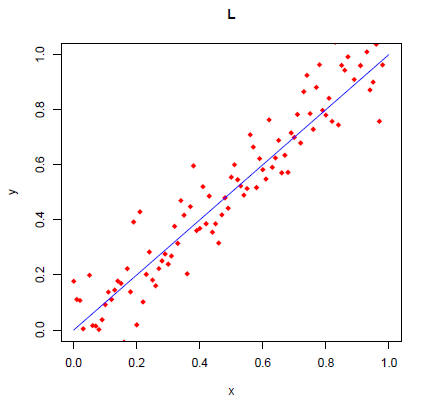
> x = seq(0,1,by=0.01) # a vector of values from 0 to 1 in
increments of 0.01.
> y = x + rnorm(length(x), mean=0, sd=0.1) # add a little Gaussian noise to x.
> plot(x,y,xlab="x",ylab="y",main="L",xlim=c(0,1),ylim=c(0,1),pch=18,col="red")
> lines(x,x,col="blue")
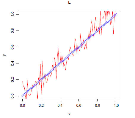
Redraw the above plot by using the type="l" option in plot
and points command
instead of line below plot.
> plot(x,y,type="l",xlab="x",ylab="y",main="L",xlim=c(0,1),ylim=c(0,1),col="red")
> points(x,x,col="blue")
Make a plot with two lines and two sets of corresponding
scatter points (similar to the
rst plot; use 4 colors): one with slope equal to one and another with slope
equal to two
using the plot, seq, points, lines and rnorm functions.
> z = 2*x + rnorm(length(x), mean=0, sd=0.5)
> plot(x,y,main="2 Lines",xlim=c(0,1),ylim=c(0,1),pch=18,col="red")
> points(x,z,pch=18,col="green")
> lines(x,x,col="blue")
> lines(x,2*x,col="purple")
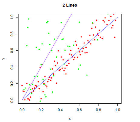
Can we see all the "green" data points? If not, how would
get them all in the plot? Try
it.
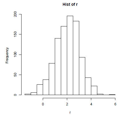
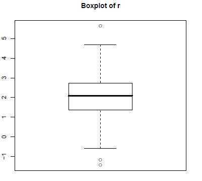
Now let's generate a plot of the histogram (using the function hist), smoothed
density
(using the function density in plot) and boxplot (using the function boxplot) of
a random
vector r which is normally distributed with a mean of 2 and standard deviation
of 1. First
we have to generate the random vector (using rnorm) and then the plots:
> r = rnorm(1000,mean=2, sd=1)
> hist(r, main="Hist of r")
> plot(density(r), "Density of r")
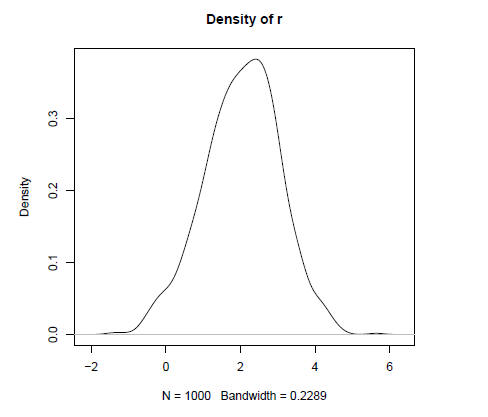
> boxplot(r, main="Boxplot of r")
7 Control Structures
R's control structures are very similar to those of other
programming languages. We will
return to our numerical vector num to illustrate the use of the if statement,
for loop and
while loop:
> if (length(num) > 2) {
+ long = TRUE
+ variance = var(num)
+ } else {
+ long = FALSE
+ variance = NA
+ }
> long
[1] TRUE
> variance
[1] 9.166667
What does the chunk of code written above do?
> squareRoot = numeric()
> for (i in 1:length(num)) {
+ squareRoot = c(squareRoot, sqrt(num[i]))
+ }
> squareRoot
[1] 3.316625 3.464102 3.605551 3.741657 3.872983 4.000000
4.123106 4.242641
[9] 4.358899 4.472136
Why did I declare squareRoot as a numeric vector before
the loop? Remove the vec-
tor squareRoot by typing rm(squareRoot) and try the loop again without declaring
the
variable. Did you get an error message? What was the problem? Could we have done
this
another, much simpler , way?
> i = 1
> sumSqrt = 0
> while (squareRoot[i] <= 4) {sumSqrt = sumSqrt + squareRoot[i]; i=i+1}
> sumSqrt
[1] 22.00092
What does the chunk of code written above do? Why did I set the variable i
before the
while loop?
8 Functions
R's strength are the thousands of powerful functions that
allow you to apply the latest
computational statistics algorithms to your data. In our case, the Bioconductor
suite of tools
is extremely powerful for array analysis and more. So, take a little time and
explore some of
the basic functions that I listed on the "R Functions and Packages" slide of the
"Introduction
to R" lecture. Use the help function to understand proper usage/input
requirements and
apply some of these basic functions to your R objects. Next, read the "Calling
Conventions
for Functions" slide to get a feel for applying a t-test and then type t.test
and read the
help page. Generate two vectors named x and y of length 10 whose elements are
normally
distributed with zero mean and standard deviation equal to one using the
function rnorm.
Next, create a vector of length 10 named z with mean two and standard deviation
one. Apply
a t.test between (1) x and y and (2) x and z using the "greater"alternative
option. Given
what you know about how you created x, y, and z, order the vectors in t.test to
yield the
lowest possible p-value.
> x = rnorm(10)
> y = rnorm(10)
> z = rnorm(10, mean=2)
> t.test(x,y,alternative="greater") # ordering doesn't matter
Welch Two Sample t-test
data: x and y
t = -0.8286, df = 14.305, p-value = 0.7895
alternative hypothesis: true difference in means is greater than 0
95 percent confidence interval:
-1.363578 Inf
sample estimates:
mean of x mean of y
-0.3222004 0.1145024
> t.test(z,y,alternative="greater") # correct ordering
Welch Two Sample t-test
data: z and y
t = 4.1771, df = 16.909, p-value = 0.0003194
alternative hypothesis: true difference in means is greater than 0
95 percent confidence interval:
1.042854 Inf
sample estimates:
mean of x mean of y
1.9020314 0.1145024
> t.test(y,z,alternative="greater") # incorrect ordering
Welch Two Sample t-test
data: y and z
t = -4.1771, df = 16.909, p-value = 0.9997
alternative hypothesis: true difference in means is greater than 0
95 percent confidence interval:
-2.532204 Inf
sample estimates:
mean of x mean of y
0.1145024 1.9020314
We'll end with learning how to write our own functions.
We're going to write a function
called medmean that calculates the median of a vector if its length is below a
user defined
value n and the mean otherwise. We'll apply it to two vectors of di erent length
which include
a bad outlier.
> medmean = function(x, n) {if (length(x) > n) {mean(x)}
else {median(x)}}
> fewdata = c(rnorm(3),100)
> manydata = c(rnorm(1000),100)
> medmean(fewdata,10) # case 1
[1] 1.411065
> medmean(fewdata,3) # case 2
[1] 25.53877
> medmean(manydata,10) # case 3
[1] 0.006908776
> medmean(manydata,1001) # case 4
[1] -0.1188903
For each of the four cases, which branch of the if
statement did we execute? Can you
draw any conclusions about applying the mean or median to data with outliers?
We'll continue next with more R and Bioconductor. Hope you had some fun learning
R.
| Prev | Next |