Real Numbers and Their Properties

Types of Numbers

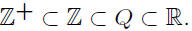
• Z⁺ Natural numbers - counting numbers -
1, 2, 3, . . . The textbook uses the notation
N.

• Z Integers - 0,±1,±2,±3, . . . The textbook
uses the notation J.

• Q Rationals - quotients (ratios) of integers.

• R Reals - may be visualized as corresponding
to all points on a number line.

The reals which are not rational are called irrational.

, the field of complex numbers , but in
this course we will only consider real numbers.

Properties of Real Numbers

There are four binary operations which take a
pair of real numbers and result in another real
number:

Addition (+), Subtraction (−), Multiplication
(× or ·), Division (÷ or /).

These operations satisfy a number of rules. In
the following, we assume a, b, c ∈R. (In other
words, a, b and c are all real numbers.)

• Closure: a+b ∈R, a · b ∈R.

This means we can add and multiply real numbers.
We can also subtract real numbers and
we can divide as long as the denominator is
not 0.

• Commutative Law: a+b = b+a, a · b = b · a.

This means when we add or multiply real numbers,
the order doesn ’t matter.

• Associative Law: (a + b) + c = a + (b + c),
(a · b) · c = a · (b · c).

We can thus write a + b + c or a · b · c without
having to worry that different people will get
different results.

• Distributive Law: a · (b + c) = a · b + a · c,
(a+b) · c = a · c+b · c.

The distributive law is the one law which involves
both addition and multiplication. It is
used in two basic ways: to multiply two factors
where one factor has more than one term and
to factor out a common factor when we add
or subtract a number of terms, all of which
contain a common factor.

• 0 is the additive identity, 1 is the multiplicative
identity.

a+0 = 0+a = a, a · 1 = 1 · a = a

• Additive Inverse: Every a ∈R has an additive
inverse, denoted by −a, such that a+(−a) = 0,
the additive identity

• Multiplicative Inverse: Every a ∈R except
for 0 has a multiplicative inverse, denoted by
a⁻¹ or 1/a, such that a · a⁻¹ = a⁻¹ · a = 1, the
multiplicative inverse.

• Cancellation Law for Addition: If a+c = b+c,
then a = b. This follows from the existence of
an additive inverse (and the other laws), since
if a+c = b+c, then a+c+(−c) = b+c+(−c),
so a+0 = b+0 and hence a = b.

• Cancellation Law for Multiplication: If a · c =
b · c and c ≠ 0, then a = b. This follows from
the existence of an multiplicative inverse for c
(and the other laws), since if a · c = b · c, then
a · c · c⁻¹ = b · c · c⁻¹, so a · 1 = b · 1 and hence
a = b.

From these rules, we can see why multiplication
by 0 gives 0: a·0+0 = a·0 = a· (0+0) =
a·0+a· 0. Thus a·0+0 = a·0+a·0 and from
the cancellation law it follows that 0 = a · 0.

We can now see why multiplication by −1 yields
the additive inverse of a number: a+(−1)·a =
1 · 1+(−1) · a = (1+(−1)) · a = 0 · a = 0.

We can also see why the product of a positive
number and a negative number must be negative,
and the product of two negative numbers
is positive. More generally, we can see that
(−a) · b = −a · b as follows: a · b + (−a) · b =
(a+(−a)) · b = 0· b = 0, so (−a) · b must be the
additive inverse of a · b, in other words, −a · b.

Subtraction and Division

All the above rules concern addition and multiplication.
Those are the basic operations; subtraction
and division are really special cases of
addition and multiplication.
Definition 1 (Subtraction). a − b = a+(−b).
Definition 2 (Division). a ÷ b = a · b⁻¹.

Alternate Notations:

This explains why division by 0 is undefined: 0
does not have a multiplicative inverse.

We also get a Cancellation Law for division: If
b ≠ 0 and c ≠ 0, then

It’s important to use the Cancellation Law correctly;
one may only cancel a factor which is
common to both the numerator and the denominator .
Often, students incorrectly try to
cancel something that is a factor of a term
of the numerator or denominator, but not a
factor of the numerator or denominator itself.

Terms and Factors

There is a technical difference between terms
and factors, and the word term is often misused
when one is actually referring to a factor.

Terms are added together.

Factors are multiplied together

x^3 + 5x^2 − 3x + 2 has four terms: x^3, 5x^2, 3x
and 2.

Technically, one might want to think of −3x
rather than 3x as the term, thinking of x^3 +
5x^2 − 3x+2 as x^3 +5x^2 +(−3x)+2, but the
common practice is to call 3x a term.

x^3 +5x^2 − 3x+2 consists of just one factor.
(x^2 + 5x − 3)(2x + 1) has just one term, but
two factors. The first factor, x^2 + 5x − 3 has
three terms and the second factor, 2x+1, has
two terms, but the entire expression, looked at
as a whole, has just one term.

The Substitution Principle

A basic principle in algebra is sometimes called
substitution. The basic idea is that, in any
algebraic expression, anthing can be replaced
by anything else that is equal to it.

This is used extensively in solving equations,
but is also used a lot in just simplifying algebraic
(and trigonometric) expressions.

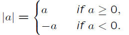
Absolute Value
Definition 3 (Absolute Value).

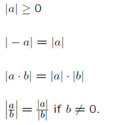
Properties of Absolute Value

Exponents

Positive integer exponents : If n ∈Z⁺, aⁿ =
a · a · a . . . a, where the product consists of n
identical factors, all equal to a.

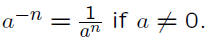
Negative exponents:

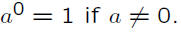
Zero exponent:

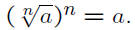
Rational Exponents: If

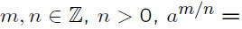
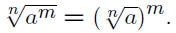
stands for the n^th root of a, the number
which, when raised to the n^th power, yields a.
In other words,

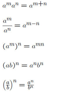
Rules for Exponents

Rules for Radicals

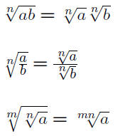
Important: We cannot simplify sums of radicals.

Order of Operations

Exponentiation
Multiplication and Division
Addition and Subtraction
If we want to change the order, we use parentheses.

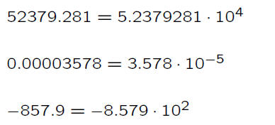
Scientific Notation

It’s sometimes convenient to write a very large
or a very small number as a number between
1 and 10 times a power of 10. This is called
scientific notation.

Examples:

Many calculators display E ± xx rather than
. For example, instead of displaying 3.578·
10⁻⁵, many calculators would show 3.578E−5.
We should still write the number down using
scientific notation, not the way the calculator
displays it.

Polynomials

Definition 4 (Polynomial). A polynomial is a
mathematical expression of the form
where
and x is a variable.

are constants and called coefficients .

a₀ is called the constant term.
a_n is called the leading coefficient.
n is the degree of the polynomial.
The variable doesn ’t have to be x.
A polynomial of degree 1 is called linear.
A polynomial of degree 2 is called quadratic.
A polynomial of degree 3 is called cubic.
Polynomials can be added and subtracted in
the obvious way.

Multiplication of Polynomials

Polynomials may be multiplied through the repeated
use of the Distributive Law, leading to
what’s sometimes called the Generalized Distributive
Law:

To multiply two polynomials together, one pairs
each term of the first factor with each term
of the second, multiplying each pair together,
and then adds all those individual products together.

Example:

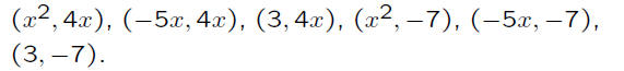
The terms of the first factor are x^2, −5x and
3, while the terms of the second are 4x and
−7. One may wish to visualize the product as
(x^2 +(−5x)+3)(4x+(−7)).

The pairs of terms may be listed, in an organized
way, in either of the following two ways:

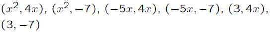
or

Using the first listing, one gets the following
products:

Adding the products together, one gets:

Combining like terms, one obtains the product:

Caution:

Many students have learned the evil acronym
FOIL. FOIL is simply the special case of the
Generalized Distribution Law for the easiest
case of all, a binomial multiplied by a binomial.
It is no easier to use than the Generalized
Distributive Law and its use detracts from
the understanding of the much more important
Generalized Distributive Law. It is advised
that students completely forget about FOIL
and avoid it at all costs.

Division of Polynomials

Division of polynomials may be done essentially
the same way long division of ordinary decimals
is performed. The most common type of division
is dividing a linear polynomial (something
in the form ax+b) into a higher degree polynomial.
Each trial quotient is obtained by dividing
the ax term into the term in the dividend
of highest degree.

When dividing a polynomial by a linear polynomial
x − c, if we get a remainder then that
remainder is actually the value of the polynomial
when x = c. We can see this if we write

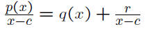
Multiplying both sides by x − c yields

p(x) = q(x)(x − c)+r

Plugging in x = c yields

p(c) = q(c)(c − c)+r = q(c) · 0+r = r.

Example: If we try dividing x^3+3x−7 by x+5
(which may be thought of as x − (−5)), we
get x^2 − 5x + 28 with a remainder of −147,
meaning that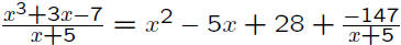
and 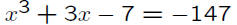when x = −5.
Corollary. Given a polynomial p(x), x − c is a
factor if and only if p(c) = 0.

This comes in very handy when solving equations.
It is the basis of solving by factoring.

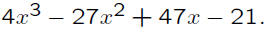
Example:

Solve x^2 +3x = 10.
x^2 +3x − 10 = 0
(x+5)(x − 2) = 0

Since x+5 and x−2 are factors, −5 and 2 are
solutions of the equation x^2+3x−10 = 0 and
thus of the equivalent original equation.

Rationalizing

Suppose one has a fractional expression like
One can rationalize the numerator as
follows:

You may remember learning to rationalize a
denominator using this method; in practice, it
turns out that one rarely if ever needs to rationalize
a denominator, but one often needs to
rationalize a numerator.

Historical Note: Before the widespread use of
calculators, rationalizing a denominator was a
useful technique to make some calculations easier.
For example, if one needed a decimal approximation
to , one used to look up a decimal
approximation to in a table, getting
1.4142 (if one was interested in four decimal
places).

Without rationalizing the denominator, one would
then have to calculate 1/1.4142 by hand, which
would be rather tedious. However, if one rationalizes
the denominator, one finds
so one could equivalently calculate
1.4142/2 by hand, a much easier calculation.

With the current availability of calculators, such
contortions are now anachronisms.

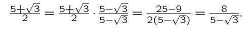
On the other hand, the skills learned in rationalizing
denominators turn out to be important
in rationalizing numerators. One example
of this is the following.

Suppose one wants to get the slope of the
line tangent to at the point (1, 1).
One can’t find it directly, but one might expect
the slope of a line between (1, 1) and a
point on the curve, close to the point
(1, 1), to be close to the slope of the tangent.

The slope of that line is , and when x
is close to 1, one expects this to be close to
the slope of the tangent. Unfortunately, it’s
hard to directly estimate the value of
However, if one rationalizes the numerator, one
observes

The last expression is obviously close to 1/2
when x is close to 1, and we thus expect the slope
of the tangent line to be 1/2, as indeed it is.

Rational Expressions

The key rules of algebra relating to rational
expressions are the following.

Cancellation Law:

(A common mistake is to think one is using
the Cancellation Law when it does not apply.)

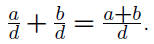
Addition:

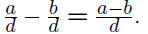
Subtraction:

(If one does not have the same denominator,
one finds a common denominator.)

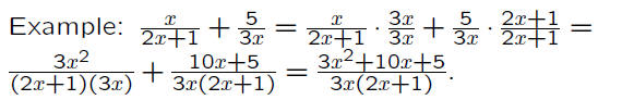
Example:

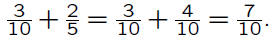
If we cannot find a common denominator easily,
we can always use the product of the denominators.
If the product isn’t the least common
denominator, we may be able to reduce
the sum we get to lower terms, cancelling a
common factor of the numerator and denominator.

Example:

We can find the least common denominator by
factoring each denominator into a product of
powers of primes and then use each prime to
the highest power it appears.

In the preceding example, the two denominators
are 4 and 6. We may factor them as:

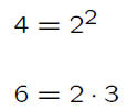
The prime factors that appear are 2 and 3.
Since the highest power 2 appears as is 2² and
the highest power 3 appears as is 3 = 3¹, the
least common denominator is 2² · 3. We may
then calculate

the same
sum we obtained before.

The same basic method may be used even if
the rational expressions involve variables.

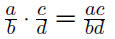
Multiplication

Division:

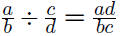
Division is really multiplication by the multiplicative
inverse of the divisor.

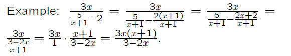
Simplifying Complex Rational Expressions

Sometimes one is confronted with rational expressions
where the numerator and/or the denominator
are themselves rational expressions.
There are two equally effective approaches to
dealing with these complex fractional expressions.

Method 1: Write the numerator and denominator
so that each is a single term, perhaps
with a numerator and denominator, and then
treat it as a quotient.

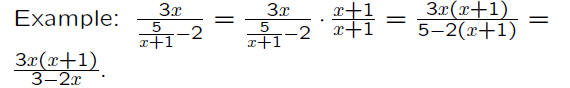
Method 2: Multiply the numerator and denominator
by the product of each factor in the denominator
of either the numerator or the denominator.