Integration of Rational Functions

In this section we will take a more detailed look at the use of partial fraction decomposi -
tions in evaluating integrals of rational functions, a technique we first encountered in the
inhibited growth model example in the previous section. However, we will not be able to
complete the story until after the introduction of the inverse tangent function in Section
6.5.

We begin with a few examples to illustrate how some integration problems involving
rational functions may be simplified either by a long division or by a simple substitution.

Example To evaluate , we first perform a long division of x + 1 into x² to

obtain

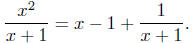
Then

Example To evaluate , we make the substitution


 

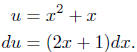
Then

Example To evaluate , we perform a long division of x + 1 into x to obtain

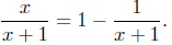
Then

Alternatively, we could evaluate this integral with the substitution

u = x + 1
du = dx.

With this substitution, x = u − 1, so we have

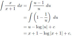
Note that this is the same answer we obtained above, although with a different constant
of integration.

Partial fraction decomposition: Distinct linear factors
Now we consider the general problem of evaluating

where both f and g are polynomials. We will assume that the degree of g is less than the
degree of f. As illustrated in the first and third examples above, if this is not the case,
we can first perform a long division to simplify the quotient into the form of a polynomial
plus a remainder term which is a rational function with numerator of degree less than the
denominator. To begin we will suppose that g factors completely into n distinct linear
factors. That is, suppose there are constants   and   such that

where the factors on the right are all distinct. From a theorem of linear algebra, which we
will not attempt to prove here, there exist constants   such that

The expression on the right of (6.4.2) is called the partial fraction decomposition of  .
Once the constants   are determined, the evaluation of

becomes a routine problem. The next examples will illustrate one method for finding these
constants.
Example To evaluate 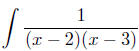, we need to find constants A and B such

that

Combining the terms on the right, we have

Now two rational functions with equal denominators are equal only if their numerators are
also equal; hence we must have

1 = A(x − 3) + B(x − 2)

for all values of x . In particular, for x = 2 we obtain

1 = −A,

from which it follows that A = −1, and for x = 3 we have

1 = B.

Thus

so

Example To evaluate 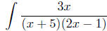, we need to find constants A and B such

that

Combining the terms on the right, we have

As before, it follows that

3x = A(2x − 1) + B(x + 5)

for all values of x. In particular, for x = −5 we obtain

−15 = −11A,

from which it follows that

and for we have

from which it follows that

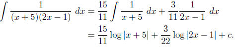
Hence

so

Partial fraction decomposition: Repeated linear factors
Returning to the general problem of evaluating

where f and g are both polynomials and the degree of f is less than the degree of g,
we will now consider the case where g factors completely into linear factors, allowing for
the possibility that one or more of these factors may be repeated. Specifically, suppose
the factor ax + b occurs n times in the factorization of g. Then the partial fraction
decomposition of must contain a sum of terms of the form

for some constants , in addition to similar terms for every other factor of g.
This is best illustrated in an example.

Example To evaluate 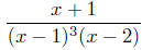, we need to find constants A, B, C, and D

such that

That is, this partial fraction decomposition contains three terms corresponding to the
factor x−1, since it is repeated three times, and only one term corresponding to the factor
x − 2, since it occurs only once. Moreover, the degrees of the denominators of the terms
for x − 1 increase from 1 to 3. Now combining the terms on the right of (6.4.4), we have

Again, it follows that

for all values of x. However, because of the repeated factors, we cannot choose values for x
which will isolate each of the constants one at a time as we did in the previous examples.
Instead, we will illustrate another technique for finding the constants. By multiplying out
(6.4.5) and collecting terms, we obtain

for all values of x. Since two polynomials are equal only if they have equal coefficients, we
can equate the coefficients of x + 1 with the coefficients of the polynomial on the right to
obtain the four equations

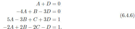
From the first equation we learn that

D = −A.

Substituting this into the second equation gives us

B = A.

Substituting both of these values into the third equation results in

C = A + 1.

Finally, substituting for D, B, and C in the fourth equation gives us

−2A + 2A − 2(A + 1) + A = 1,

which gives us A = −3. Hence B = −3, C = −2, and D = 3. Thus

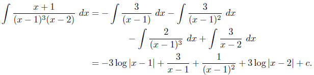
Note that in solving for A , B, C, and D, we could have first substituted x = 1 and x = 2
into (6.4.5) to obtain values for C and D, respectively. These values could have then been
used to simplify (6.4.6) before solving for A and B.

The Fundamental Theorem of Algebra states that every polynomial factors into a
product of linear factors and irreducible quadratic factors ; hence, to complete the story of
integrating rational functions, we need to consider the case where the factorization of the
denominator includes irreducible quadratic factors. However, we will learn in Section 6.5
that for an irreducible quadratic polynomial g,

involves the inverse tangent function. Thus we need to discuss the inverse trigonometric
functions before continuing the story of integrating rational functions.

Problems

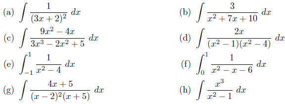
1. Evaluate each of the following integrals.

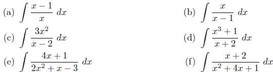
2. Evaluate each of the following integrals.

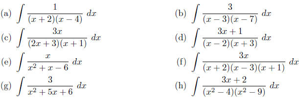
3. Evaluate each of the following integrals.

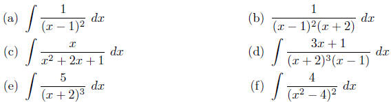
4. Evaluate each of the following integrals.

5. Solve the differential equation

using the method used to solve the logistic differential equation in Section 6.3. Assume
x(0) = 0 and −1 < x(t) < 1 for all t.