Linear Algebra
Due Today. Exercises from section 1.1, page 8,
numbers 1–4, 13–14, 21–22, 23, and T4.
Read for Friday. Finish 1.2 on matrices and
read 1.3 on dot products and matrix multiplication.
Due Friday. Exercises from section 1.2: 1–2, 4–7
parts a–d each, 8, 9, T1, T5a.
No class Monday. Martin Luther King Jr. Day.
Due Wednesday. Exercises from section 1.3: 1–
4, 7, 9, 11–12, 19–20, 33, T1, T4, ML1, ML2, ML5,
ML6ac.
The ML exercises are Matlab exercises. Do
them, but you don’t have to make printed versions
of them. Feel free to use Matlab to help you
with your homework, even the parts of Matlab
we haven’t discussed in class.
Last time. We discussed systems of linear equations.
Sometimes they’ve got exactly one solution,
sometimes no solutions, and sometimes infinitely
many solutions. We saw the method of elimination
as the ancient Chinese did it, how they created a
matrix from the system of linear equations , first
put the matrix into echelon form, then into reduced
echelon form, and then they could read the solution
right from the resulting matrix.
We’ll formalize this method soon.
Today. We’ll review some of the topics in section
1.1 about linear systems , and we’ll begin discussing
section 1.2 which introduces matrices.
Standard notation and terminology. When
we’ve got a system of linear equations, we’ll usually
let m denote the number of equations , and n
the number of variables, and say the system is a
m× n system of equations. For instance, here’s an
example 3 × 2 system of equations:

Here, m = 3 since there are 3 equations, and n = 2
since the two variables are x and y . (Typically,
when a system has more equations than unknowns ,
then there are no solutions. Does this system have
any solutions?)
When there are many variables, we usually subscript
them, but when there are few variables we
ususally use different letters for the variables. For
instance, if n = 6, we might use the 6 variables
 , and
, and  ,
but if n = 3, we might use
the three variables x, y, and z.
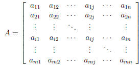
A general m × n system looks like this :

where the n variables are
 . The m
constants that appear on the right side of the m
equations are denoted  . Since each of
the m equations has n coefficients for the n variables,
there are mn coefficients in all, and these are
denoted with doubly subscripts, so, for instance

is the coefficient of the variable  in the
third equation.
A solution to the system is an n-tuple of values
for the n variables that make all the equations simultaneously
true. For example, in the 3×2 system
above, a solution is (x, y) = (2, 1). In fact, it’s the
only solution for that system.
Matrices. A matrix is a rectangular array of
numbers. You can see how they’re related to systems
of equations since the system is determined
by its coefficients and its constants, and those can
naturally be displayed in a matrix. Consider the
3 × 2 system of equations above. Its coefficients
can be displayed in the 3 × 2 matrix

called the coefficient matrix for the system. If you
want to include the constants a a matrix, too, you
can add another column to get the 3 × 3 matrix

called the augmented matrix for the system. Frequently,
a vertical line is added to separate the coefficients
from the constants, as in

Standard terminology and notation for matrices.
When a single symbol is used to denote
an entire matrix, it’s usually a capital letter, like A
or B.
Usually m is used for the number of rows and
n for the number of columns. Such a matrix is
called an m × n matrix. When m = n we say the
matrix is a square matrix . When symbols are used
for the elements (that is, entries) of a matrix, they
are often doubly indexed (that is, subscripted), and
the indices indicate where the entry is located. For
instance,  indicates the element in the 3rd
row
and 4th column. Note that the first index gives the
row number and the second index gives the column
number. When a generic row is needed, usually i is
used, and when a generic column is needed, usually
j is used. So  is the element in the ith row
and
jth column.

Special square matrices. Square matrices were
mentioned above. There are some special square
matrices we’ll discuss in class including diagonal
matrices, scalar matrices, and the identity matrix.
A square matrix for which  = 0 whenever i ≠
j
is called a diagonal matrix. The main diagonal of
a square matrix consists of the elements  .
The
.
The
main diagonal is usually just called the diagonal.
Thus, a diagonal matrix only has nonzero entries on
its diagonal. If all the entries of a diagonal matrix
are the same, it’s called a scalar matrix. The most
important scalar matrix has all 1’s on its diagonal,
and that matrix is called an identity matrix, and
it’s usually denoted I. Thus, an identity matrix
has 1’s on its diagonal and 0’s elsewhere.
Some of the homework exercises talk about
upper-triangular matrices and lower-triangular matrices.
Row and column vectors. If a matrix has only
one row, that is, if m = 1, then we’ll call it a row
vector. Likewise, if it has only one column, that is,
if n = 1, then we’ll call it a column vector.
Equality of matrices. Two matrices are equal
when they have the same shape and all their corresponding
entries are equal.
Addition and subtraction of matrices. If two
matrices are the same shape, then you can add
them together to produce another matrix by adding
the corresponding elements together. Likewise you
can subtract one matrix from another if they have
the same shape. Examples 11 and 13 in the text
illustrate when these operations are useful .
Scalar multiplication. The word “scalar” in
this subject means “number,” and by that we usually
mean real number . Later in the course we’ll
take our field of scalars to be the field of complex
numbers or some other field. For now we’ll stick to
reals. We’ll use the standard notation R for the set
of all real numbers (that is, all positive numbers ,
negative numbers , and 0).
Scalar multiplication is an operation where you
can multiply a scalar and a matrix together. It’s
done by multiplying every entry in the matrix by
that scalar. For instance, if A is a matrix, then 2A
is found by doubling every entry in A. Note that
2A = A+A, just as you would expect. Also, when
A and B are two matrices , then A−B = A+(−1)B,
just as you would expect.
Linear combinations. In mathematics, you say
that a linear combination of things is a sum of multiples
of those things. So, for example, one linear
combination of the matrices A, B, and C is
2A+3B−4C. In other words, a linear combination
of matrices is found by the operations of addition,
subtraction, and scalar multiplication.
The transpose of a matrix. One more simple
operation we can discuss now is transposition. It’s
where you exchange rows and columns in a matrix.
For instance, if A is the matrix
 ,
,
then the transpose of A, denoted AT is the matrix
 .
.
Note that if A is an m×n matrix, then its transpose
AT is an n × m matrix. Also note that the transpose
of the transpose is the original matrix, that
is (AT )T = A. Also, note that transposition turns
row vectors into column vectors, and vice versa.
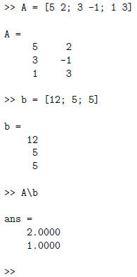
Matrices in Matlab. Last time we saw how
easy it was to enter into Matlab the coefficient
matrix A and constant column vector b of a system
of linear equations, and then compute the solution.
Let’s see what Matlab does for the 3 × 2 system
of equations above.

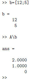
Let’s try Matlab on this system


Thus, (x, y, z) = (2, 1, 0) is a solution to the system
of equations. But it’s not the only solution.
Another is (x, y, z) = (3,−7, 11), and there are infinitely
more solutions to this indeterminate system.
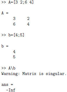
On the other hand, the system

is inconstant, that is, it has no solutions. Matlab
gives


We’ll see later how Matlab can be used to help
you find all the solutions to a system.
Matlab also allows you to do create the identity
matrices of various sizes, do addition and subtraction
on matrices of the same shape, multiply a
scalar and a matrix, take a transpose of a matrix,
as well as many other operations, most of which
we’ll use throughout the course.


| Prev | Next |