Matrix Introduction and Operations
1 Matrix operations
1.1 Introduction
Matrix notation is a way of representing data and equations. An example from
Bronson (1995):
T-shirts
Nine teal small and five teal medium; eight plum small and six plum medium;
large sizes- three
sand, one rose, two peach ; also three medium rose, five medium sand, one peach
medium, and seven
peach small.
In a matrix the same information looks like this:
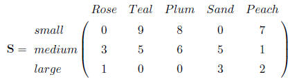
In this format, it is easy to understand and work with the information. By
summing each column
we can tell how many of each color there are, and by summing each row we can
tell how many of
each size there are.
Matrices are made up of elements arranged in horizontal rows and vertical
columns. The size of a
matrix is given as rows × columns, for example the t-shirt matrix is 3 × 5. A
vector is a matrix
with 1 row × any number of columns or 1 column × any number of rows.
The matrix itself is usually capitalized, and the elements of the matrix are
referred to in lower case
letters with row and then column in subscript. In the above matrix S each
element sij corresponds
to the element in the ith row and jth column, with sij representing the number
of small teal shirts.
Matrices are often expressed as capital and bold typed latin letters, whereas
vectors most often are
expressed as bold lower case latin letters.
1.2 Matrix Addition
Matrices can be added together or subtracted from one another if the
dimensions of the two matrices
are the same. If this is true, then each element of the matrix is added to its
corresponding element
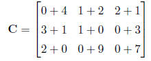
in the other matrix. Subtraction works similarly. For example, if matrix A
is
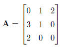
and matrix B is
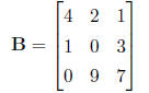
then matrix C = A + B is defined as
A natural extension of matrices to programming is through arrays.
2-dimensional arrays are analogous
the matrices shown here, but because arrays are not actually matrices, matrix
operations
have to be specified in most general programming languages.
Algorithm 1 Matrix Addition
if A and B are both n × p matrices then
for i = 1 to n do
for j = 0 to p do
Cij = Aij + Bij
end for
end for
end if
1.3 Matrix Multiplication
Matrix multiplication is less intuitive than matrix addition. First, the
matrices have to be of defined
proportions . Matrices of different sizes can be multipled as long as the number
of columns in the
first matrix equals the number of rows in the second matrix. The formal
definition of this is that
any matrix of n rows ×p columns can be multiplied by any matrix of p rows ×r
columns, where
the resulting matrix is n rows ×r columns. Second, the actual operations are
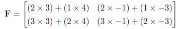
defined differently . If

and matrix E is
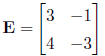
then matrix

is defined as
This becomes more clear when we are working with linear equations . Linear
equations can be
written as:
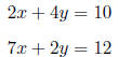
Or, in matrix-vector notation:
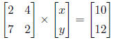
Now it is a little easier to see how to multiply the matrices and vectors, and what the result is.
1.4 The Lande Equation
An example of where this is used in evolution is the Lande equation and
G-matrices. Lande (1979)
defined the phenotypic response to selection as
 . This means that the per-generation
change ( )
in a phenotypic trait (z) is equal to the additive genetic variance (G)
multiplied by
)
in a phenotypic trait (z) is equal to the additive genetic variance (G)
multiplied by
Algorithm 2 Matrix Multiplication C = AB
if A is an n × p and B is p × r then
for i = 1 to n do
for j = 1 to r do
for z = 1 to p do
cij = aizbzj + cij
end for
end for
end for
end if
the selection on that trait (β), or the partial
derivative of mean fitness with respect to the trait
 (Lande
and Arnold 1983). If we expand this to multiple phenotypic traits we can write
the
(Lande
and Arnold 1983). If we expand this to multiple phenotypic traits we can write
the
response to selection as a vector of changes in phenotypic traits. The matrix G
contains the additive
genetic variances for each trait on the diagonal and the genetic covariances
between traits
are the off-diagonal elements. To find the response to selection, we multiply
this G matrix by the
selection vector.
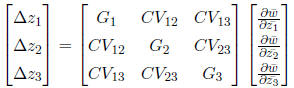
The system can be represented in matrix-vector notation, but can also be
split into three separate
equations.
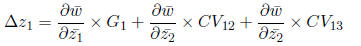
Looking at it this way, we can see that the change in each trait is found by
summing the selective
forces caused by selection on the trait itself and correlated effects from
selection on other traits.
1.5 Matrix Transposition
A matrix can be transposed from A to AT by converting all the columns of
matrix A to the rows of
matrix AT and the rows of matrix A to the columns of matrix AT . The first row
of A becomes the
first column of AT , and so on. The definition of this is if A is an n×p matrix,
then the transpose
of A is denoted by AT and is defined as AT (j, i) = A(i, j).
Algorithm 3 Matrix Transposition A -> AT
for i = 1 to n do
for j = 1 to m do
AT (j, i) = A(i, j)
end for
end for
1.6 Matrix Inversion
If we have a system of linear equations Ax = b, we might like to solve for x .
In an algebraic equation
this would happen by dividing both sides by A but in matrix algebra division is
undefined. Instead,
we use matrix inversion. A matrix A-1 is defined as the inverse of
matrix A if

where I is the identity matrix. I is defined as a square matrix with all
diagonal elements equal to
one and all off-diagonal elements equal to 0. In order to satisfy this, both
matrices must be square
and of the same order. If there is no matrix A-1 that satisfies this
condition the matrix is singular.
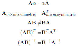
Multiplication of a square matrix with its inverse is commutative
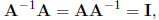
but multiplication of two different (square) matrices A and B is not

here an example of an inversion:
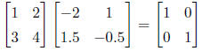
Matrix inversion can be used in the Lande example to solve for
β, the
selection vector. The inverse
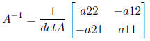
of a 2×2 matrix is found with the determinant, defined as a11×a22 - a12×a21. The
inverse is:
The Lande equation specifies that at equilibrium the change in the trait will
be zero , or
 .
If
.
If
we have biased mutation (w) or some other force acting on the system, we can
express it as:
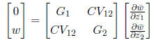
To solve for β at equilibrium, we multiply both sides by the inverse matrix
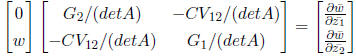
And we can now solve for each βi.
1.7 Vector and matrix norms
A Norm is a measure of distance. We can apply norms to vectors and matrices.
1.7.1 Vector norms
Requirements for vector norms are:
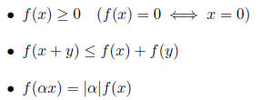
f(x) is the vector norm and is expressed typically as
||x||. Several vector norms are often used.
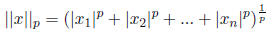
The general expression is sthe p-norm. It is expressed as
Of these the 1,2, and  norms are the most commonly used ones:
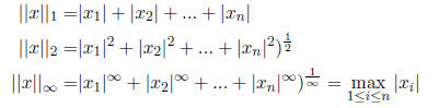
the 1-norm is also called Manhattan distance or city block
distance and the 2-norm is the Euclidian
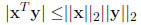
distance. Vector norms have some cool properties for example the
 inequality:
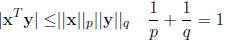
A special case is the Cauchy-Schwartz inequality
Several more inequalities can be used to approximate or
bound norms, but you might want to look
into the book by Golub and van Loan (1996).
1.7.2 Matrix norms
Matrix norms are an important measure to assess whether
they are fit for some operations, matrix
norm can measure whether a matrix is near singularity. Matrix norms need the
same requirements
as the vector norms. Examples for matrix norms are the Frobenius-norm

and the p-norm
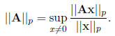
Think of sup as the maximum, at least for real numbers .
the matrix norms often can be broken
down into vector norms.
1.8 Summary of matrix operations not explicitely discussed
1.9 Sources and Additional Reading
Bronson, R. 1995. Linear Algebra: An Introduction. San
Diego, CA, Academic Press.
Golub, G. H., and C. F van Loan 1996. Matrix computations. 3rd edition. John
Hopkins University
Press, Baltimore and London.
Lande, R. 1979. Quantitative-genetic analysis of multivariate evolution, applied
to brain-body size
allometry. Evolution 33: 402416.
Lande, R., and S. J. Arnold. 1983. The measurement of selection on correlated
characters. Evolution
37:12101226.
Trefethen, L.N. and D. Bau, III. 1997. Numerical Linear Algebra. Philadelphia,
PA, Society for
Industrial and Applied Mathematics .
| Prev | Next |