Thank you for visiting our site! You landed on this page because you entered a search term similar to this: solving non-linear simultaneous equations two variables excel, here's the result:
Guided tour on VAR innovationresponse analysis
Introduction
In this guided tourI will explain how to conduct vector autoregression (VAR) innovation responseanalysis, including structural vector autoregression innovation responseanalysis.The theory involvedin explained in my lecturenotes (VAR.PDF) on vector time series and innovation response analysis,but here I will review the main ideas, based on the seminal papers:
- Bernanke, B.S. (1986):"Alternative Explanations of the Money-Income Correlation", Carnegie-RochesterConference Series on Public Policy 25, 49-100
- Sims, C.A. (1980):"Macroeconomics and Reality", Econometrica 48, 1-48
- Sims, C.A. (1986):"Are Forecasting Models Usable for Policy Analysis?", Federal ReserveBank of Minneapolis Quarterly Review, 1-16
Xt= c0 + C1Xt-1 + .....+ CpXt-p + Ut ,
where
- Xt= (X1,t, ..... ,Xk,t)' is avector time series of macroeconomic variables,
- c0is a k-vector of intercept parameters,
- the Cjare k´kparameter matrices, and
- Utis the error vector, which is assumed to be i.i.d. k-variate normallydistributed with expectation the zero vector, and variance matrix S.
C(L)Xt= c0 + Ut,
where
is a matrix-valued lag polynomial, with L the lag operator: LXt= Xt-1.
The process Xtis strictly stationarity if det[C(z)] has all its roots outsidethe complex unit circle. Then C(L) is invertible, i.e., thereexist k´kparameter matrices Dj, with D0= Ik and åj³0DjDj'a finite matrix, such that
C(L)-1= åj³0DjLj.
Hence, the processXthas a stationary MA(¥)representation:
Xt= m + åj³0DjUt-j,
where m= (åj³0Dj)c0.Note that E[Xt] = mand Var[Xt] = åj³0DjSDj'.
Since the Ut'sare i.i.d. with E[Ut] = 0, it follows now thatfor m ³0:
E[Xt+m|Ut]- E[Xt+m] = DmUt.
The latter isthe basis for innovation response analysis, i.e., E[Xt+m|Ut]- E[Xt+m] is the net effect of the innovationUton the future values Xt+m of Xt.
Non-structural VAR innovationresponse analysis
Sims (1980) proposesto interpret the components of the innovation vectorUt= (U1,t, ..... ,Uk,t)' as policy shocks. The problemhowever is that the components U1,t, ..... ,Uk,tof Ut are not independent, so that it is unrealisticto assume that a shock in one of these components does not affect the othercomponents. In order to solve this problem, Sims (1980) proposes to rewriteUtasUt= Det,
where Dis a lower triangular matrix such that
S= DD'.
Then etis i.i.d. Nk[0,Ik]. The componentse1,t,..... ,ek,t of et are uniquely associatedto the corresponding components of Ut. Consequently,we can now interpret e1,t, ..... ,ek,tas the actual innovations, and moreover we may consider them as sequentialpolicy shocks: at time t a shock e1,t is imposed,and after then the next shock e2,t is imposed, etc., up to the lastshockek,t. Then the response of Xtto a unit shock in ej,t is:
E[Xt+m|ej,t= 1] - E[Xt+m] = Dmdjfor m = 0,1,2,3,.....,
where djis column j ofD,and thus the response of Xi,t to a unit shock in ej,tis given by
ri,j(m)= E[Xi,t+m|ej,t = 1] - E[Xi,t+m]= di,m'djfor m = 0,1,2,3,.....,
where di,m'is row i of Dm.
Structural VAR innovation responseanalysis
A disadvantage ofthis approach is that economic theory plays a limited role. The only roleof economic theory is to determine the order in which the innovationshocks are imposed. This order corresponds to the order in which the macroeconomicvariables in Xt are arranged. Therefore, Bernanke (1986)and Sims (1986) propose to set up the VAR(p) model as a system ofsimultaneous equations:B.Xt= a0 + A1Xt-1+ ..... + ApXt-p + et,
where etis i.i.d. Nk[0,Ik]. The matrix Brepresents the contemporaneous relations between the components of Xt.This structural VAR(p) model is related to the non-structural VAR(p)model
Xt= c0 + C1Xt-1+ ..... + CpXt-p + Ut ,
by
Xt= B-1a0 + B-1A1Xt-1+ ..... + B-1ApXt-p + B-1et,
Hence, c0= B-1a0,Cj = B-1Ajfor j = 1,..,p, andUt = B-1et.The latter reads as
B.Ut= et.
Therefore, effectivelythe matrix B of structural parameters links the nonstructural innovationsUtto the structural innovations et.
The main differencewith the non-structural approach is the way the variance matrix Sof Ut is decomposed, i.e., instead of writing Ut= Detwith D a lower triangularmatrix we now have Ut = B-1et,hence S = (B-1)(B-1)'= (B'B)-1, and thus
B'B= S-1.
Given S,and taking into account the symmetry of S,the equality B'B = S-1is a system of (k + k2)/2 nonlinear equationsin thek2 elements of B. Therefore, in order tosolve this system, one has to set at least (k2 - k)/2off diagonal elements of B to zeros, similarly to classical simultaneousequation systems. This is where economic theory comes into the picture:The zeros in B are exclusion restrictions prescribed by economictheory.
Note thateven if we reduce the system B'B = S-1to (k + k2)/2 equations in (k + k2)/2unknowns, there is no guarantee that there exists a solution, because theequations involved are quadratic. But assuming that we have spread thezeros in B such that a solution exists, the structural innovationresponse of Xi,t to a unit shock in ej,tis given by
ri,j(m)= E[Xi,t+m|ej,t = 1] - E[Xi,t+m]= di,m'bjfor m = 0,1,2,3,.....,
where againdi,m'is row i of Dm, and bjis now column j of B-1.
Estimation and inference
The non-structuralVAR(p) model can be estimated by maximum likelihood. Given the maximumlikelihood estimators of the coefficient matrices Cjfor j = 1,..,p, and the variance matrix S,and the joint normal asymptotic distribution of the parameters therein,it is possible to derive asymptotic standard error of each innovation responseri,j(m).EasyReg International endows the estimated innovation responses involvedwith one and two times standard error bands based on the asymptotic normaldistribution of each estimated innovation response around the true innovationresponse, in order to determine whether the latter is significantly differentfrom zero. The two-times standard error band corresponds approximatelyto the pointwise 95% confidence interval of each innovation response. Theone-time standard error band corresponds approximately to the pointwise70% confidence interval.EasyReg Internationalestimates a structural VAR model in three steps. First, the non-structuralVAR is estimated by maximum likelihood. Next, given the estimated variancematrixS and the specificationof the matrix B, EasyReg will try to solve the nonlinear equationssystem B'B = S-1analytically, and if this is not possible, it will minimize the maximumabsolute value of the elements of the matrix B'B -S-1.The latter is a form of method of moments estimation. Finally, using thenon-structural parameter estimates and the solution of B as startingvalues, EasyReg re-estimates the parameters by maximum likelihood. Giventhese maximum likelihood estimates, the innovation responses and standarderror bands are computed in the same way as in the non-structural case.
Note that directmaximum likelihood estimation of the structural VAR model (as some othereconometric software packages do) is not advisable because the likelihoodfunction is highly nonlinear in the non-zero elements of B, andtherefore you may get stuck in a local maximum.
VAR innovation response analysiswith EasyReg
The data
The data are taken from the EasyReg database, namely the following quarterly data for the US: Since VAR innovation response analysis assumes normal errors of the VAR, and the variables involved are all positive valued, transform them by taking logs, using the 'Transform variables' option via Menu > Input: The last three variables are likely nonstationary. Therefore, take them in firstdifferences, using the option Menu > Input > Transform variables > Time series transformations.Then select the variables in Xt = (X1,t,X2,t,X3,t,X4,t)'in the following order: for t = 1,2,...,142, from quarter 1959.2 (t = 1) to quarter 1994.3 (t = 142). The transformed data are also available in Excel 97 workbook formatVAR.XLS and CSV (US number setting) format VAR.CSV.
VAR model specification
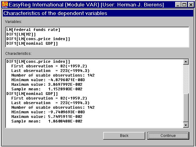
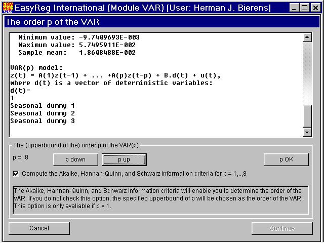
OpenMenu > Multiple equations models > VAR innovation response analysis, select the variablesin the VAR in the above order, and click "Selection OK". Then the followingwindow appears. I will not select a subset of observations. Thus click "No" and then "Continue": This window is only for your information. Click "Continue": In the introduction above I have discussed only a VAR model with interceptparameter vector c0. However, if Xt (= z(t) in EasyReg) is stationary around a deterministic function of time,i.e., Xt - E[Xt] isstationary, we can still conduct VAR innovation response analysis. The VAR(p) model then takes the form: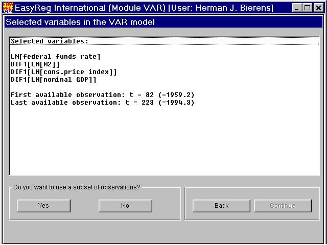
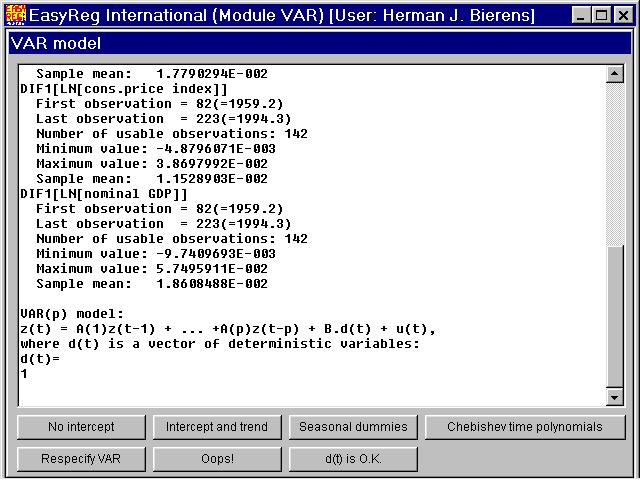
Xt= C0d(t) + C1Xt-1 + .....+ CpXt-p + Ut ,
where d(t) is a vector of deterministic functions of timet, and C0 (= B in EasyReg) is the corresponding matrix of coefficients. Note that
The default specification of d(t) is d(t) = 1. Other options are d(t) = (1,t)', seasonaldummy variables (only in the case of seasonal data, of course), and Chebishevtime polynomials. The latter can be used to capture nonlinear time trends. TheChebishev time polynomials have been used in my paper
- Bierens, H.J. (2000), "Nonparametric Nonlinear Co-Trending Analysis, with an Application to Inflation and Interest in the U.S.", Journal of Business & Economic Statistics 18, 323-337,
It is logically impossible that the (transformed) data contain a linear time trend, because that would imply that the expectation of some of the variables involved converge to plus or minus infinity.
Since the data are quarterly data, and because it is not clear whether the dataare seasonally adjusted, I recommend to include in first instance seasonal dummy variables, next to the constant 1. Whether seasonal dummy variables are neededcan be tested. Thus click "Seasonal dummies":
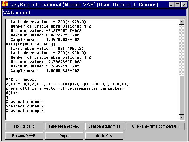
Note that only three quarterly dummies are included next to the contant 1, because the four seasonal dummies add up to 1 and would thereforebe perfectly multicollinear with 1.
Now click "d(t) is OK":
There are various ways to determine the order p of theVAR(p) model
Xt= C0d(t) + C1Xt-1 + .....+ CpXt-p + Ut.
Via this window you can determine p automatically by one of three information criteria:
- Akaike = ln[det(S)] + 2[1/(n-p)].(m+p.k2)
- Hannan-Quinn = ln[det(S)] + 2.[ln(ln((n-p))) / (n-p)].(m+p.k2)
- Schwarz = ln[det(S)] + 2 .[ln(n-p)/(n-p)].(m+p.k2)
Another way to determine p is through testing the joint significance of the parametersin the matrices Cj. I will consider this later.
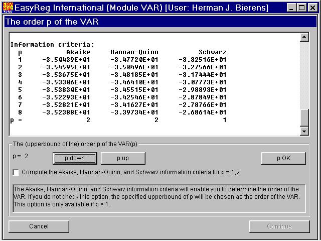
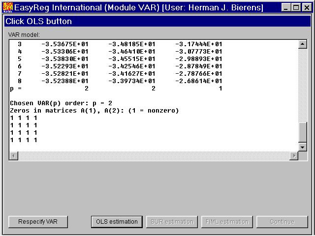
In view of these results, I have chosen p = 2.
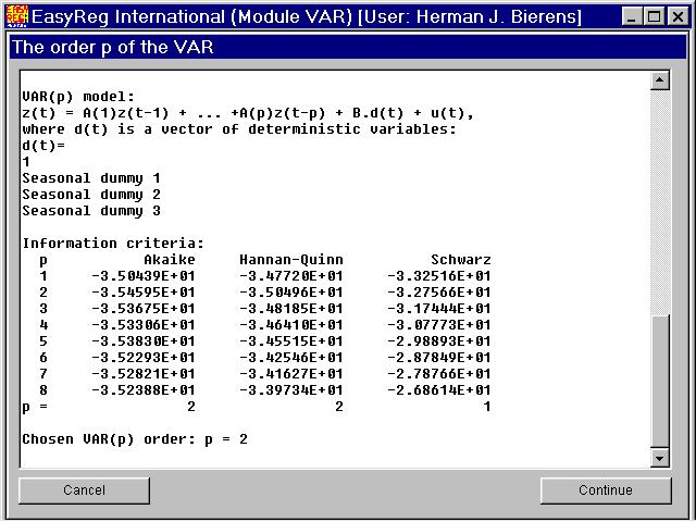
This window is only for your information. Click "Continue".
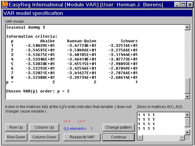
This window enables you to impose Granger-causality restrictions on the VAR. See my lecturenotes (VAR.PDF) on vector time series and innovation response analysis.Granger-causality will be discussed below by a separate example. Thus, click "Continue".
Since each equation in the VAR model
Xt= C0d(t) + C1Xt-1 + .....+ CpXt-p + Ut, t = p+1,...,n,
has the same right-hand side variables, andthere are no parameter restrictions imposed, the maximum likelihood estimatorsof the parameters in the matrices Cj for j = 0,1,...,pare the same as the OLS estimators. Thus, click "OLS estimation" first. After EasyRegis done with OLS estimation, the button "FIML estimation" will be enabled. FIML standsfor Full Information Maximum Likelihood. Given the vectorsRt of OLS residuals, the maximum likelihood estimator of the variance matrix S of the VAR error vector Ut is
Sn = (n-p)-1p+1 t nRtRt',
which is decomposed as
where Dn (= L in EasyReg) is a lower triangular matrix. We need FIML in order to compute the variance matrix of the non-zeroelements of Dn, which in its turn is needed tocompute the standard error bands of the innovation responses. Thus, click "FIML estimation" when it becomes enabled. Then the following window appears.
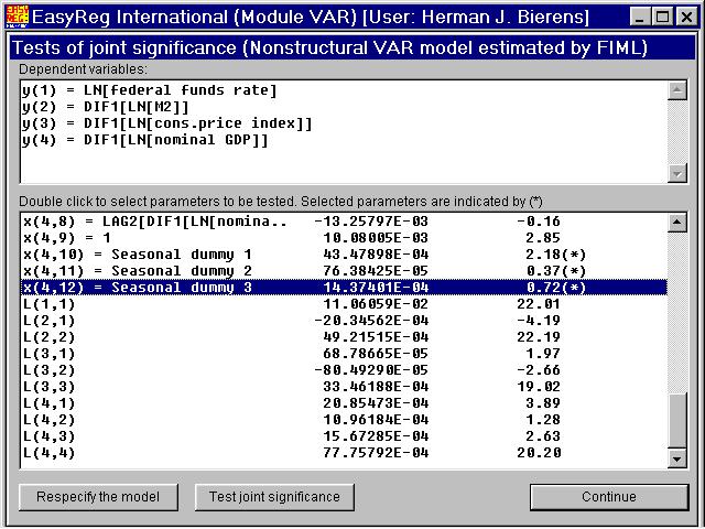
The variables L(.,.) are the non-zero elements of the lower triangular matrix Dn (= L).
You can now test the joint significance of any subset of parameters of the VAR. First, I havetested the joint significance of the parameters of the seasonal dummy variables: Double-clickthe seasonal dummies (note that each of the four equations contains three seasonal dummy variables, so that you have to double-click all 12 seasonal dummy variables), and thenclick "Test joint significance":
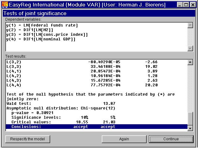
The test involved is the Wald test of the null hypothesis that all the coefficientsof the seasonal dummy variables are zero. The asymptotic null distribution isc2 with 12 degrees of freedom. Clearly, the nullhypothesis involved is not rejected at any conventional significance level.
In view of this result, we may now respecify and re-estimate the VAR without seasonal dummy variables. However, I have not done that.
If you click "Again", you can conduct more tests.
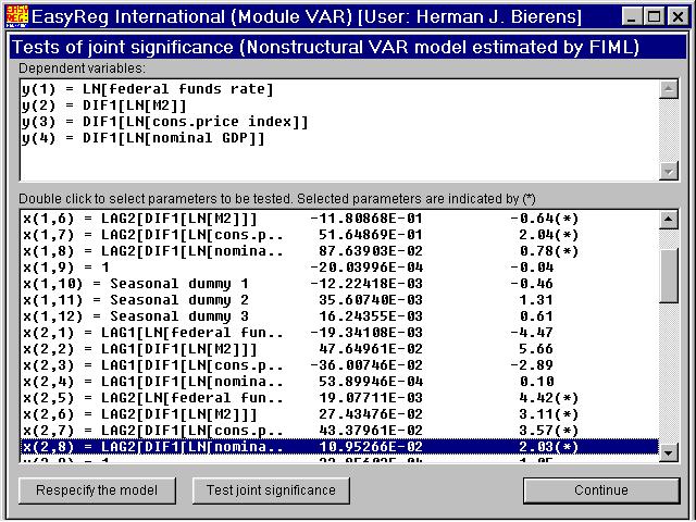
Next, I have tested whether the VAR order p can be reduced from p = 2 to p = 1, by testing whether the 16 coefficients corresponding to the variables with lag 2 (i.e., the elements of the matrix C2) are jointly zero.
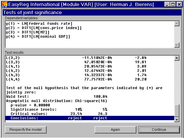
Clearly, the null hypothesis involved is rejected. Therefore I will adopt the initial choice p = 2.
Note that this procedure is an alternative way to determine the VAR order p. Given an initial value of p for which you are convinced that the actualVAR order does not exceed this initial value,test whether the elements of the matrices Cj for j = q,...,p (with q 1)in the VAR model
Xt= C0d(t) + C1Xt-1 + .....+ CpXt-p + Ut
are jointly zero, and take as the new p the largest value of q for which thishypothesis is rejected.
Now click "Continue". Then the following windows appears.
Let us conduct non-structural VAR analysis first. After you are done with that, you will return to this window so that you can conduct structural VAR analysis. The sameapplies the other way around.
Non-structural VAR innovationresponse analysis
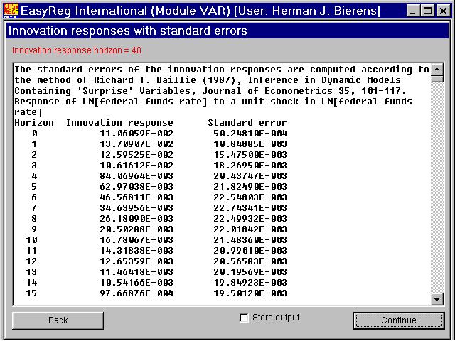
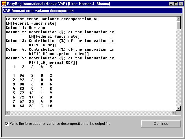
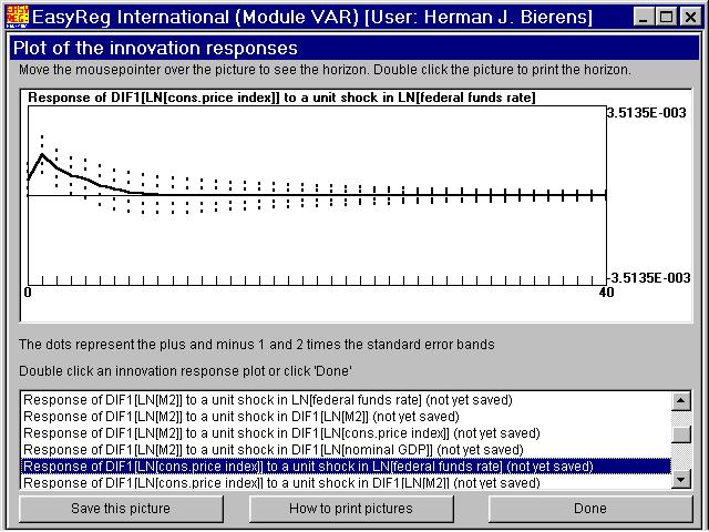
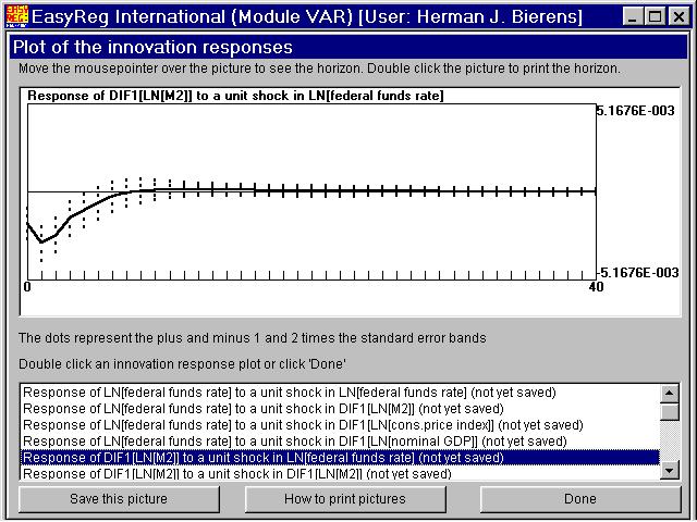
You have to choose the number of periods ahead (the innovation response horizon) for which you want to display the innovation responses. The minimum value is 10. HereI have chosen 40, so that the innovation responses are displayed over a period of 10 years. Click "Start" to compute the innovation responses together with their standard errors. You will have the option to write the numerical values of the innovation responses withtheir standard errors to the output file OUTPUT.TXT, but in general there is no purposein doing this. Thus, click "Continue". The contribution of the innovation in variable i to the h-step ahead forecast error of variable j is the sum of the squared responses of variable j to a unit shock in the innovation of variable i. In this window the relative contributions of each variable i to the forecast error variance of variable j are presented. This procedure is known as "variance decomposition". Click "Continue". The solid curve is the response of the inflation rate to a unit shock in the innovation of the log of the federal funds rate. You see that in the first three quarters the response is significantly positive, as the two-times standard error band is above thehorizontal axis, and then dies out quickly to zero. This phenomenon is known as the price puzzle. Since the FED raises the federal funds rate in order to curtail inflation,one would expect that the response of inflation to a unit shock in the innovation of thefederal funds rate is negative rather than positive. This picture is the response of the money growth rate to a unit shock in the innovation of the log of the federal funds rate. This pattern is what you would expect: Ifborrowing money is made more expensive, the demand for money will decrease. When you click "Done", EasyReg will jump back to the the following window.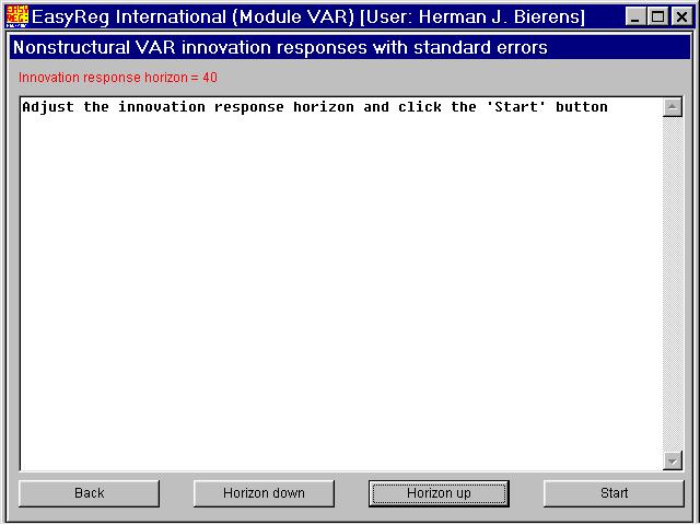
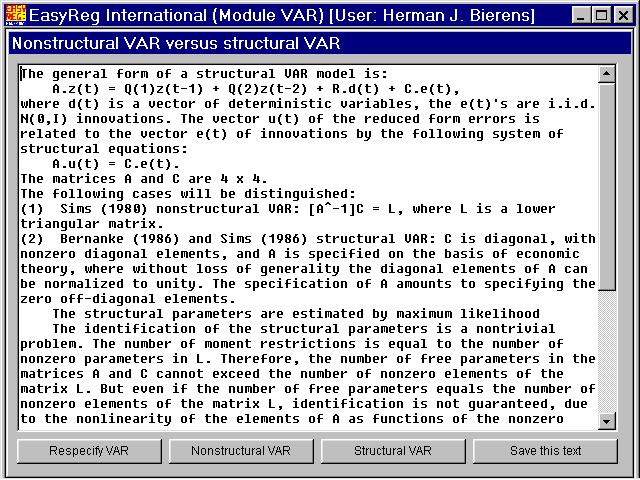
Structural VAR innovationresponse analysis
The matrice A in the description of the structural VAR is a matrix of structuralparameters with ones as diagonal elements, and the matrix C is a diagonal matrix. Thesematrices are related to the matrix B in the structural model
B.Xt= a0 + A1Xt-1+ ..... + ApXt-p + et,
used in the previous discussion of structural VAR analysis by the equality
Recall that the structural model relates the nonstructural VAR errors Utto the structural VAR errors et by the relationships
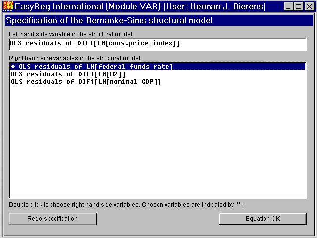
In the following four windows the non-zero elements of each row of B arespecified.
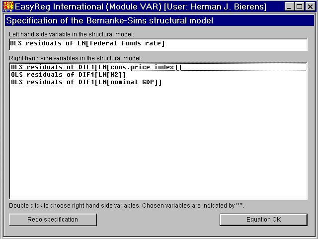
The first element on row 1 of B is always non-zero. The remaining three non-zeroelements are determined by double-clicking the correponding components of Ut. In this example I will choose the first row of B to be (b(1),0,0,0), hence I will not double-click anything, but just click "Equation OK".
I will choose (b(2),b(3),0,0) as the second row of B.The second element b(3) of row 2 is always non-zero, and b(2) is the coefficient ofthe non-structural innovation in the log of the federal funds rate. Thus, double-clickthe latter, and click "Equation OK".
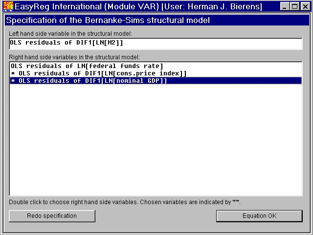
When you click "Equation OK", (0,b(4),b(5),b(6)) will be chosen as the third rowof B.
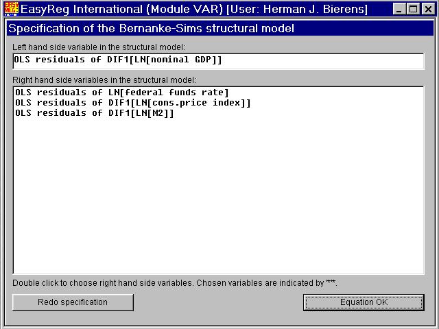
Finally, when you click "Equation OK", (0,0,0,b(7)) will be chosen as the fourth rowof B. Then the matrix B is:
b(1) 0 0 0 b(2) b(3) 0 0 0 b(4) b(5) b(6)0 0 0 b(7)
Note that this specification is not intended to be a serious economic specification,but is chosen merely as an example.
EasyReg will now try to solve the equation system B'B = Sn-1 analytically:
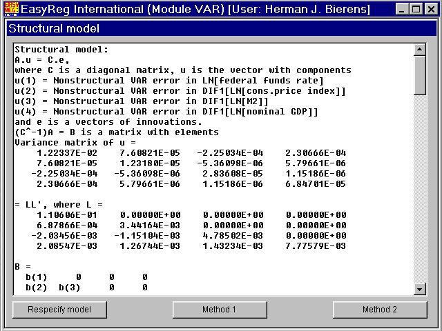
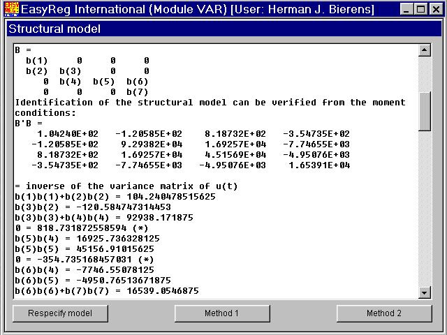
What you see here is equations in the systemB'B = Sn-1. The equation indicated by (*) does not involve parameters, because the system is over-identified:there are more equations than unknown b(.).
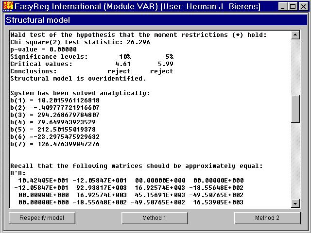
The equation in the previous window indicated by (*) is a testable hypothesis. In this examplethe null hypothesis that the equation holds is rejected, hence we should respecifythe matrix B. However, since this is only a demonstration of structural VAR analysis, Iwill continue.
Note that the non-zero parameters in B are solved analytically.
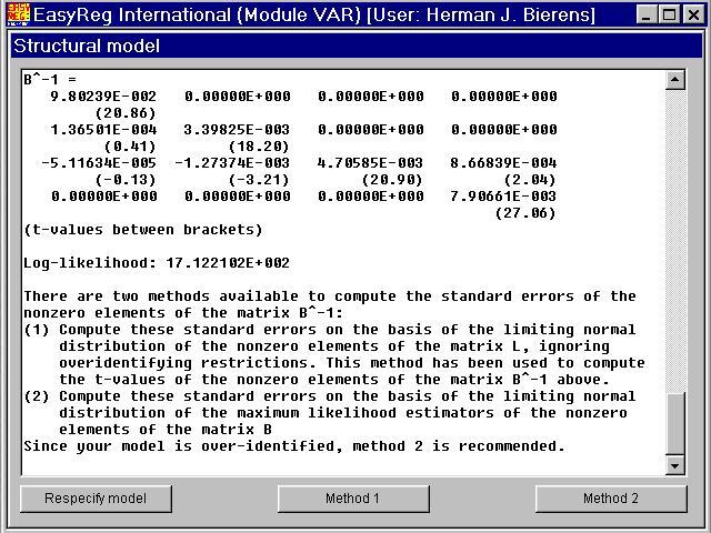
Click "Method 2". Then the maximum absolute value of the elements of the matrixB'B - Sn-1(called MAD: The Maximum Absolute Deviation of the elements of B'B from the corresponding elements of Sn-1)will be minimized, using the simplex method of Nelder and Mead.
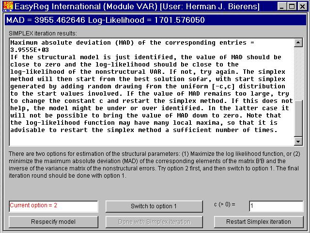
Next, switch to Option 1. Then the non-zero elements b(1),...,b(7) of B will be estimated by maximum likelihood, starting from the previous solutions.
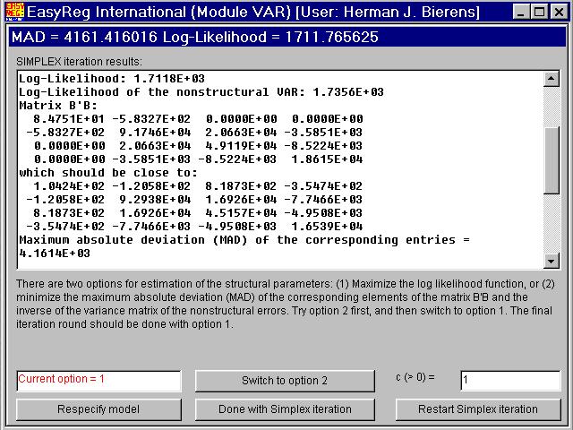
When you click "Done with Simplex iteration" the following window appears.
From this point on structural VAR analysis is similar to the non-structural case.
Granger-causality
Introduction
Consider a bivariate time series process Xt =(X1,t,X2,t)'.As is well-known (or should be well-known), the best one-step ahead forecast of each componentXi,t of Xt is the conditional expectation
i.e., of all functions of the past of Xt, saygi(Xt-1,Xt-2,Xt-3,.....),this conditionalexpectation yields the smallest mean-square forecast error:
Now suppose that
Then the past of the process X2,t does not contain information thatcan be used to improve the forecast of X1,t. If so, it is saidthat X2,t does not Granger-cause X1,t (called after Clive Granger at UCSD who introduced this causality concept).
If Xt is a VAR(p) process:
Xt= c0 + C1Xt-1 + .....+ CpXt-p + Ut ,
and X2,t does not Granger-cause X1,t, then the matrices Cj for j = 1,...,p are lower-triangular, becausethe coefficients of the lagged X2,t in the VAR are zero.
Granger-causality testing in practice
Retrieve two annual time series from the EasyReg database, namely LN[nominal GDP], which is the log of nominal GPD of the US, and LN[Income Sweden], which is the log of national income of Sweden. Then use thetransformation option (via Menu > Input > Transform variables > Time series transformations) totransform these time series in first differences, in order to make them stationary:
- DIF1[LN[nominal GDP]]
- DIF1[LN[Income Sweden]]
Now plot them (via Menu > Data analysis > Plot time series):
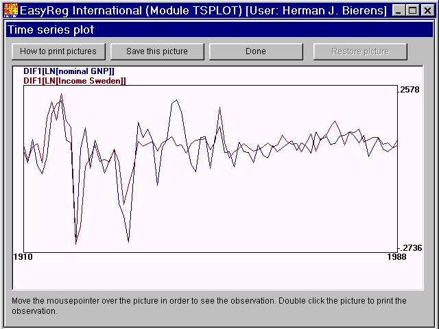
You see that these time series have quite a few similar patterns. The reason is that due to the size of the US economy theUS GDP growth rate may be considered as a proxi for the world economic growth rate. Sweden is a small country and its economic performance heavily depends on exports. Therefore,the US GDP growth rate will affect the Swedish national income growth rate, but not the other way around. In other words, one may expect that DIF1[LN[Income Sweden]]does not Granger-cause DIF1[LN[nominal GDP]]. To test this, select these variablesin the above order in a VAR:
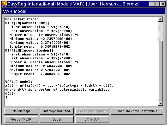
It is clear from the plot that there is no time trend in these series, and you see inthis window that the averagegrowth rates (= sample means) are non-zero. Therefore, include only intercepts in the VAR. Thus,click "d(t) is OK":
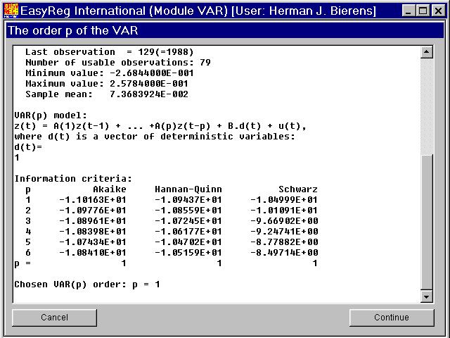
I have chosen p = 6 as the initial value of p. The three information criteriaall indicate that the actual value is p = 1. Therefore, I have chosen p = 1.
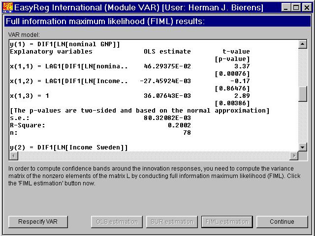
The coefficient of one year lagged DIF1[LN[Income Sweden]] in the equation forDIF1[LN[nominal GDP]] has t-value -0.17, and is therefore not significant. Consequently, the null hypothesis that DIF1[LN[Income Sweden]] does notGranger-cause DIF1[LN[nominal GDP]] is not rejected at any conventialsignificance level.
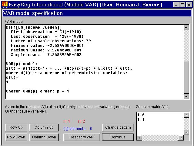
In order to impose this restriction on the VAR(1), click "Respecify VAR", select the two variables again, and choose p = 1:

The VAR(1) involved is now of the formXt = a0 + A1Xt-1+ Ut, whereXt = (X1,t,X2,t)'with
- X1,t = DIF1[LN[nominal GDP]]
- X2,t = DIF1[LN[Income Sweden]]
a 0b c
say, which corresponds to the pattern
1 01 1
Therefore, click "Column Up", and then "Change pattern":
Click "Continue":
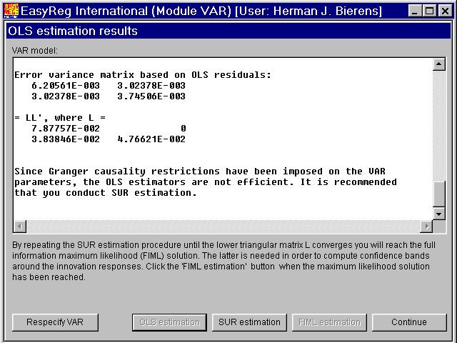
First, click "OLS estimation" in order to get initial estimates. Since there are parameterrestrictions imposed on the VAR, OLS is no longer efficient. Therefore, after OLS is done, thebutton "SUR estimation" becomes enabled. SUR stands for Seemly Unrelated Regression. SUR estimation of the restricted VAR(1) modelXt = a0 + A1Xt-1+ Ut involves the following steps:
First, estimate the variance matrix S of Ut onthe basis of the vector of OLS residuals. Denote this variance matrix estimate bySn,0. Second, maximize the likelihood functionL(a0,A1,S)to a0 and A1, with Sreplaced by Sn,0.Third, re-estimate S on the basis of the new estimates of a0 and A1. Denote this estimate by Sn,1. The new estimates of a0 and A1 are efficient, in the sense that the limitednormal distribution of the parameters therein is the same as for the maximum likelihood estimators,but the estimator Sn,1 may not yet be efficient.Therefore, I recommend that you repeat the steps 2 and 3, each time j replacing Sn, j-1 with Sn, j, until these matrices converge:
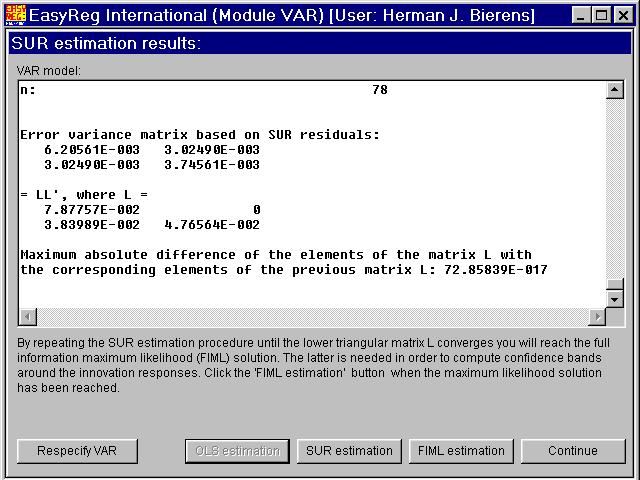
In each SUR estimation step j the matrixSn, jis decomposed as asSn, j= Ln, jLn, j',whereLn, j is a lower triangular matrix, and themaximum absolute deviation of the non-zero elements of Ln, j from the corresponding elementsof Ln, j-1 is computed. If the lattergets small enough, continue with full information maximum likelihood estimation. Thus,click "FIML estimation", and then "Continue":
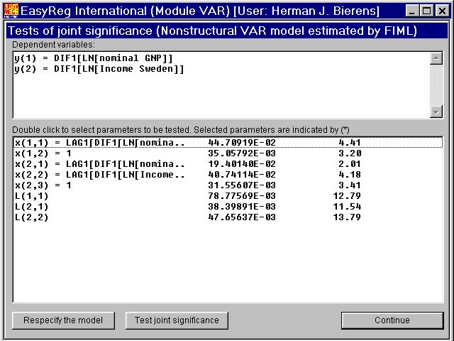
You can now conduct joint significance tests.
Click "Continue", choose "Non-structural VAR", and innovation response horizon = 10:
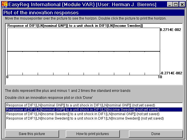
Since DIF1[LN[Income Sweden]] does notGranger-cause DIF1[LN[nominal GDP]], the innovation responses involved are all zero.
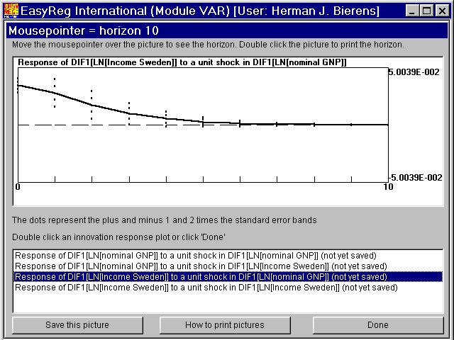
On the other hand, a unit shock in the innovation of DIF1[LN[nominal GDP]] hasa significant positive impact on DIF1[LN[Income Sweden]], at least in the first threeyears after the shock in the innovation of DIF1[LN[nominal GDP]].
VAR models with exogenous variables: VARX models
In principle it is possible to include exogenous variables in a VAR model, next to determinsitic variables such as trends, and conduct innovation response analysis via EasyReg. How to do that is explained in PDF file VARX.PDF.
This is the end of the guidedtour on VAR innovation response analysis.