Bayesian Inference for Global Sensitivity Analysis of Radiative Transfer Models

Introduction

• Global process models are widely used in geoscience and remote sensing for the estimation and
prediction of the properties of Earth’s coupled dynamical system. Such models are typically implemented
in complex computer programs that require global inputs.

•We are concerned with Radiative TransferModels (RTMs), which simulate light reflected off the surface
of the earth. RTMs are typically computationally expensive, and while they are deterministic
models, there is uncertainty about the true values of their inputs.

•We use the Leaf-Canopy Model (LCM) as a surrogate for the RTM, and study the sensitivity of
the LCM’s output to uncertainty in its inputs using global sensitivity analysis. Then, we determine
inputs that are most influential with regard to the LCM output prediction uncertainty.

Leaf-Canopy Model

• The LCM was developed in support of MODIS (or Moderate Resolution Imaging Spectroradiometer),
a key instrument abroad Terra and Aqua satellites, in order to capture essential biophysical
processes associated with the interaction between light and vegetation.

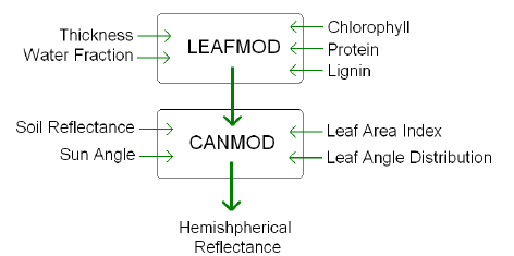
• The LCM combines two radiative transfer algorithms: LEAFMOD, which simulates the radiative
regime inside the single leaf, and CANMOD, which combines the information coming from LEAFMOD
with canopy structural parameters to compute the radiative regime within and at the top of
the canopy.

Figure 1: The inputs and output of the coupled algorithm of the LCM

• Input variables: We set the leaf angle distribution to planophile (leaves mostly horizontal) and
the sun angle to zenith, and consider chlorophyll, water fraction, thickness, lignin, protein, Leaf
Area Index (or LAI), and soil reflectance, denoted by

•Output: y = f (v) is hemispherical reflectance, which is the LCM output given inputs v.

Global Sensitivity Analysis

• The influence of each input and how uncertainty in the output is apportioned amongst the inputs
are determined by calculating the “main effects” and “sensitivity indices” of the LCM inputs.

• Output function Decomposition:

• The global mean is given by , where H (v) is the distribution of the
inputs. Based on related literature, we use independent uniforms over the ranges of the inputs.

• The main effects are given by
where v_−i denotes all the elements of v except v_i. The later terms of the decomposition are the
interactions, which give the combined influence of two or more inputs taken together.

• Assuming independence between the input variables in the uncertainty distribution, H(v), the total
variance, Var(Y ) = W, can be decomposed as the sum of partial variances,

and analogously for the higher order terms.

• The sensitivity indices, are given by

where S_i is the first-order sensitivity index, S_ij, for i ≠ j, is the second-order sensitivity index,
and so on. We’re interested in S_i, which measures the fractional contribution of v_i to Var(Y ).

• Another important sensitivity measure is the total sensitivity index,
where W_−i is the total contribution to the variance of f(v) due to all inputs except v_i.

• Computing the main effects and sensitivity indices requires the evaluation of multidimensional integrals
over the input space of the model. The LCM is computationally expensive, so obtaining
these quantities through Monte Carlo methods using LCM runs is not feasible.

• Using a Bayesian approach, we approximate the LCM with a Gaussian Process (GP) emulator and
efficiently obtain posterior inference for the main effects and sensitivity indices.

Bayesian Gaussian Process Emulator

• A GP is a stochastic process that places a probability distribution over a function, f(·), such
that given a finite set of input points, , the joint probability distribution of
is multivariate normal.

• A GP is fully specified by its mean function, μ (v), and covariance function,
. We assume a constant mean, μ, and an isotropic covariance function with constant
variance,, and correlation function,

•We use the GP to formulate a prior distribution for the function f(v). Then, using a small number
of carefully chosen RTM runs, we obtain a posterior distribution according to Bayes’ Rule using
Markov chain Monte Carlo (MCMC) sampling.

• The main effects and sensitivity indices of the LCM inputs are then obtained using computationally
“cheap” runs of the the GP posterior.

Results

•We construct the Bayesian GP emulator using a training set of 250 LCM runs based on a Latin
hypercube design at 8 MODIS spectral bands that are sensitive to vegetation.

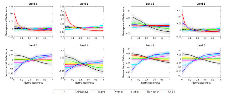
Figure 2: Medians ( smooth lines ) and 95% probability bands (the shaded regions around the
medians) of the posterior distributions of main effects of the LCM at 8 different MODIS bands.

• Normalizing the inputs allows all the main effects to be plotted together on the same plot. The
larger the variation of the main effect plot, the greater the influence of that input on the LCM output.
The slope of each main effect plot gives information as to whether the output is an increasing
or decreasing function of that input.

• For visible spectrum (bands 1, 2, & 6), the LCM is most sensitive to chlorophyll, and an increase in
chlorophyll results in a decrease in the LCM output. For red light (band 6), LAI becomes important
as well, and an increase in LAI results in a decrease in the LCM output.

• For near infra-red (bands 3, 7, & 8), the LCM is most sensitive to LAI, lignin, and thickness (in
that order), and an increase in LAI or thickness produces an increase in the LCM output, while an
increase in lignin produces a decrease in the LCM output.

• For short infra-rad bands (bands 4 & 5), LAI and lignin continue to be influential inputs, with water
fraction also becoming influential. An increase in LAI produces an increase in the LCM output,
while an increase in lignin produces a decrease in the LCM output.

Figure 3: The distributions of the first-order sensitivity indices (in magenta) and the total
sensitivity indices (in cyan) of the LCM inputs as estimated by the GP emulator.

• The box plots of the sensitivity indices show that inputs with influential main effects also have large
sensitivity indices, which means they are major contributors to the variation in the LCM output.

•Many inputs with negligible ( nearly zero ) first-order sensitivity indices had non-negligible total
sensitivity indices. A substantial difference between the first-order sensitivity index and total sensitivity
index of a particular input implies an important role of interaction terms involving that
input on the variation in the output.

• For all 8 MODIS bands, we find that interaction terms involving the 7 LCM inputs are influential in
controlling output variability, which indicates that the dimension of the LCM input is irreducible.

Discussion and Future Work

•We have implemented a Bayesian approach, via MCMC methods for the GP emulator, to obtain
posterior inference for the main effects and sensitivity indices associated with the 7 LCM inputs at
8 different MODIS bands.

• Our analysis enabled the identification of influential first-order effects of the inputs to the LCM and
revealed that interaction terms are also important in controlling the variation of the LCM output.

•We plan to study a Bayesian variable selection approach in the context of sensitivity analysis, where
the GP correlation parameters are used to make screening decisions in order to reduce the input
space by identifying “active” inputs.

• The long-term goal is to validate the LCM using field data, and to invert the LCM in order to obtain
the distribution of Leaf Area Index, a key input to global climate models, over large geographic
regions, given measured reflectances from the satellite data.

Acknowledgements:
This work was supported in part by the NASA AISR program through grant number
NNX07AV69G.