
ERROR AND SENSITIVITY ANALYSIS FOR SYSTEMS OF LINEAR EQUATIONS
ERROR AND SENSITIVITY ANALYSIS FOR SYSTEMS OF LINEAR EQUATIONS
| • Read Sections 2.7, 3.3, 3.4, 3.5. • Conditioning of linear systems . • Estimating accuracy • Error analysis |
Perturbation analysis Consider a linear system Ax = b. The question addressed by perturbation analysis is to determine the variation of the solution x when the data, namely A and b, undergoes small variations. A problem is ill-conditioned if small variations in the data lead to very large variation in the solution.  Let E, be an n × n matrix and e be
an n-vector. “Perturb” A into A(ε) = A +
εE and b into b + εe. Note: A + εE is nonsingular for ε small enough. Let E, be an n × n matrix and e be
an n-vector. “Perturb” A into A(ε) = A +
εE and b into b + εe. Note: A + εE is nonsingular for ε small enough. Why? The solution x (ε) of the perturbed system is s.t. Why? The solution x (ε) of the perturbed system is s.t.
|
||||
Let  . Then, . Then, x(ε) is differentiable at ε = 0 and its derivative is x(ε) is differentiable at ε = 0 and its derivative is
|
The quantity  is called the
condition is called the
conditionnumber of the linear system with respect to the norm  . When . Whenusing the standard norms  , we label κ(A) , we label κ(A)with the same label as the associated norm. Thus,  Note: Note:
 ratio of largest to ratio of largest tosmallest singular values of A . Allows to define  when A is when A isnot square . Determinant *is not* a good indication of sensitivity Small eigenvalues *do not* always give a good indication of poorconditioning.
|
||||
Example: Consider matrices of the form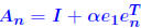 for large α. The inverse of  is is and for the ∞-norm we have  so that  For a large α, this can give a very large condition number, whereas all the eigenvalues of are equal to unity. |
Rigorous norm-based error bounds First need to show that A+E is nonsingular if A is nonsingular and E is small: LEMMA: If A is nonsingular and  then A + E then A + Eis non-singular and  Proof is based on expansion  THEOREM 1: Assume that (A + E)y = b + e and Ax = b and that . Then A + E is nonsingular and
|
||||
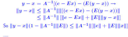
| roof: From (A + E)y = b + e and Ax = b we get A(y − x) = e − Ey = e − Ex − E(y − x). Hence:
Note: stated in a slightly weaker form in text.
Assume that
|
Another common form : THEOREM 2: Let (A + ΔA)y = b + Δb and Ax = b where  , and assume that , and assume that . Then . Then
|
||||
| Normwise backward error Question: How much do we need to perturb data for an approxi- mate solution y to be the exact solution of the perturbed system? Normwise backward error for y is defined as smallest ε for which  Denoted by  . y is given (some computed solution). E and e are to be selected . y is given (some computed solution). E and e are to be selected(most likely ’directions of perturbation for A and b’). Typical choice: E = A, e = b Explain why this is not unreasonable
|
Let r = b − Ax. Then we have: THEOREM 3:  Normwise backward error is for case E = A, e = b:  Show how this can be used in practice as a means to stop some Show how this can be used in practice as a means to stop someiterative method which computes a sequence of approximate solutions to Ax = b. Consider the
6×6 Vandermonde system Ax = b where   . We perturb A by E, with . We perturb A by E, with|E| ≤ 10−10|A| and b similarly and solve the system. Evaluate the backward error for this case. Evaluate the forward bound provided by Theorem 2. Comment on the results. |
||||
| Componentwise backward error A few more definitions on norms... A norm is absolute
 for all x. (satisfied by all for all x. (satisfied by allp-norms). A norm is monotone if
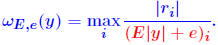
 . It can be shown that these two properties are equivalent. . It can be shown that these two properties are equivalent.... and some notation:  (where E ≥ 0, e ≥ 0) is the componentwise backward error. |
Show: a function which satisfies the first 2
requirements of vector norms (1.  (==0, iff x = 0) and 2. (==0, iff x = 0) and 2.
  satisfies the triangle inequality iff its unit ball is convex. Use the above to construct a norm in R2 that is satisfies the triangle inequality iff its unit ball is convex. Use the above to construct a norm in R2 that is*not* absolute. Define absolute *matrix* norms in the same way. Which of theusual norms  , and , and
 are absolute? Recall that for any matrix fl(A) = A+E with are absolute? Recall that for any matrix fl(A) = A+E with
 . .For an absolute matrix norm  What does this imply? |
||||
THEOREM 4 [Oettli-Prager] Let r = b − Ay
(residual). Then
|
is equal to
|
||||
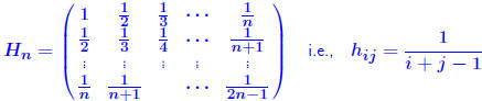
| Example of ill-conditioning: The Hilbert Matrix Notorious example of ill conditioning.
|
Estimating Condition numbers. Let A,B be two n ×
n matrices with A nonsingular and B singular. Then 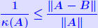 Proof: B singular →:  x ≠ 0 such that Bx = 0. x ≠ 0 such that Bx = 0. Divide both sides by  result. result.QED. Example: let 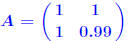 and and
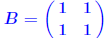 Then  . . |
||||
| Estimating errors from residual norms Let  an approximate solution to system Ax = b (e.g., computed an approximate solution to system Ax = b (e.g., computedfrom an iterative process). We can compute the residual norm:  Question: How to estimate the error  from from
 ? One option is to use the inequality ? One option is to use the inequality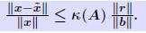 We must have an estimate of κ(A). We must have an estimate of κ(A). |
Proof of inequality. First, note that  . So: . So: Also note that from the relation b = Ax, we get  Therefore,  Show that Show that
|
||||
| THEOREM 6 Let A be a nonsingular matrix and
an
approximate solution to Ax = b. Then for any norm , In addition, we have the relation  in which κ(A) is the condition number of A associated with the norm . It can be shown that
|
Iterative refinement Define residual vector: We have seen that: We have seen that:
 , i.e., we have , i.e., we have Idea: Compute r accurately (double precision) then solve Idea: Compute r accurately (double precision) then solve ... and correct by ... repeat if needed. |
||||
|
ALGORITHM : 1 Iterative refinement Do { 1. Compute r = b − A 2. Solve  3. Compute  } while  Why does this work? Model: each solution gets m digits at most because of the conditioning: For example 3 digits. At the first iteration, the error is roughly  . Second iteration: error in . Second iteration: error in
 is roughly is roughly
 . (but now . (but now is much smaller than is much smaller than
 ). ).etc .. |
Iterative refinement - Analysis Assume residual is computed exactly. Backward error analysis: So:   A previous result showed that if  then then So : process will converge if (suff. condition) So : process will converge if (suff. condition) |
||||
| Important: Iterative refinement won’t work when
the residual r consists only of noise. When b − Ax is already very small (≈ ε) it is likely to be just noise, so not much can be done because 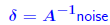 Heuristic: If ε = 10−d, and  then each iterative then each iterativerefinement step will gain about d − q digits. A matlab experiment [do operations indicated ]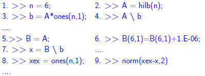 |
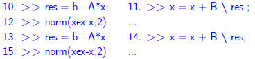 repeat a couple of times.. Observation: we gain about 3 digits per iteration. Read Section 3.5.4 on estimating accuracy. |
||||



 :
:

 and
and
 and
and
 then
then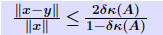

 ,
,




 .
. .
. .
. into 0.20001.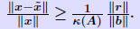

| Prev | Next |