Basic Operations on Matrices
In this worksheet you’ll find Maple commands used in
matrix manipulation.
Definitions and rules of matrix operations can be found in section 7.2.
Notes: before you can use these matrix commands you have to bring up
the package linalg (for LINear ALGebra) using the with
command.
> with(linalg):
Warning, new definition for norm
Warning, new definition for trace
1. Define a matrix:
You can use the command matrix to declare a matrix in Maple. Basically,
you must tell Maple the size of the matrix ( number of rows and then number
of columns) and the values of its entries (in row order).
Example: Let’s define a matrix A of size 3x4 (three rows and 4 columns).
> A:= matrix(3,4,[-1,1,0,0,2,-2,0,2,3,3,10,9]);

Example: You can think of a vector in Rˆn as a
matrix of n rows and one
column.
> vec:= matrix(4,1,[1,2,3,4]);

2. Addition and multiplication by a scalar:
Remember that you can add or substract two matrices only if they are of
the same size (same numbers of rows and same numbers of columns). You can
also multiply a matrix by any scalar (real or complex number).
These operations are componentwise !
Example: Let B be a matrix of size 3x4 (the same size as that of A given
above)
> B:= matrix(3,4,[-2,3,2,0,1,2,0,1,1,2,-1,2]);

Then we can compute: A+B, A-B, 3*A, A-2*B by using
the command
evalm (EVALuate Matrices) as follows
> AplusB:= evalm(A+ B); AminusB:=evalm(A-B); threexA :=evalm(3*A);\
Aminus2B:=evalm(A-2*B);
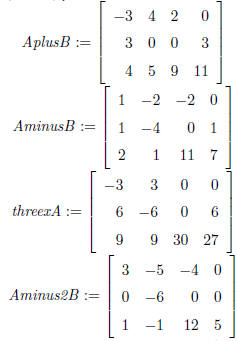
Note: all the results above have the same size
(3x4) as those of A and B.
3. Multiplication of matrices:
You can compute C*D where C and D are two matrices if and only if
the number of columns of C equal the number of rows of D
For example: We cannot have A*B because #cols of A=4 and #rows of
B=3.
However, if C is a matrix of size 4x2 then we can compute A*C and the
result is a matrix of size 3x2 (#rows = #rows of A; #cols = #cols of C).
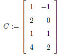
Example: Lets define a matrix C of size 4x2 and compute A*C (can we
compute C*A? why not?)
> C:= matrix(4,2,[1,-1,2,0,1,1,4,2]);
> AC:= multiply(A,C);

Instead of using the command multiply to compute
the product A*C we
can use again the command evalm to get the same thing. However, we
have
to use the operation &* in this command to tell Maple that this is a
matrix multiplication.
> evalm(A &* C);

Notes: if A and B are square matrices (#rows=#cols)
of the same size
then we can compute both A*B and B*A. However, A*B are not equal to
B*A in general. That is: matrix multiplication is not a commutative
operation.
4. Determinant:
If A is a square matrix , we can compute its determinant by using the
command det
> A:= matrix(3,3,[1,2,3,2,-2,1,0,2,4]); detA:= det(A);

detA := −14
5. Inverse of a square matrix:
If A is a square matrix then its inverse (if exists!) is the square
matrix B
of the same size such that the product A *B and B*A are the identity matrix.
If the inverse of A exists we say that A is invertible.
Important:
A square matrix is invertible if and only if the determinant of A is
nonzero
For example, the matrix A defined above is invertible.
We can compute the inverse of A by using the command inverse of Maple.
> invA:= inverse(A);
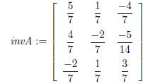
Let’s check if the product A*invA and invA*A are both
identity matrix (you
can also use the command evalm).
> multiply(A,invA); mult2iply(invA,A);

6. Matrix function:
Each entry of a matrix can be a function and we can perform differentiation
and integration operation on the matrix. Again, these operations are simply
componentwise.
Example: Let f be a matrix 2x2 whose entries are functions in t
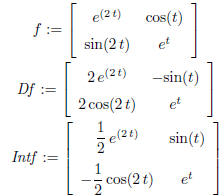
> f:=matrix(2,2,[exp(2*t),cos(t),sin(2*t),exp(t)]);
We compute the derivative of f with respect to the argument t. Thing is
a little bit complicate here because we cannot simply type diff(f,t).
Maple
requires us to use the command map for this kind of operation (In other
words,
we have to map the procedure diff to all matrix entries).
> Df:= map(diff,f,t);
Compute the integral of f (again, using the map command to map the
procedure int to all matrix entries).
> Intf:=map(int,f,t);
Eigenvalues and Eigenvectors
The background material for this part is presented in section 7.3.
Given a square matrix M. For example
> M:= matrix(3,3,[1,0,4,4,1,-2,5,0,2]);

We define the characteristic matrix ofMto be the
matrix lambda*Identity
- M. That is
> Id:=matrix(3,3,[1,0,0,0,1,0,0,0,1]); cM:=evalm(lambda*Id-M);
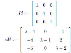
The Maple command charmat can be used to get the
same result
> charmat(M,lambda)2;

The characteristic polynomial of M is simply the
determinant of the
characteristic matrix. For example,
> cpoly_of_M:= det(cM);

You can also use the command charpoly to compute the characteristic
polynomial of a matrix M. For example,
> charpoly(M,lambda);

The eigenvalues of the matrixMare simply the roots of this polynomial .
> evs:= solve (cpoly_of_M=0,lambda);
evs := 1, 6, −3
You can also use the command eigenvals to compute these values
> evs:= eigenvals(M);
evs := 1, 6, −3
There are eigenvectors of the matrix M corresponding to each of the eigen-values.
An eigenvector of M corresponding to the eigenvalue r is a vector X
such that M*X = r*X
Equivalently , X is the solution of the system (r*Id -
M)*X=0. We say that
X belongs to the nullspace of the matrix r*Id-M.
For example, if we want to compute eigenvectors of the matrix M corresponding
to the eigenvalue 6 then we have to compute the nullspace of the matrix
6*Id - M. The Maple command nullspace can be used here
> m:=evalm(6*Id-M); nullspace_of_m:=nullspace(m);
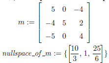
That is, the eigenvector corresponding to 6 is (10/3, 1,
25/6).
Similarly, we can compute the eigenvectors corresponding to the other
eigenvalues
1,-3.
The command eigenvects can be used to get all the eigenvectors of
the
matrix M at one shot:
> eigenvects(M);

In this case we have three lists. Each of them tells us:
the eigenvalue, its
multiplicity (how many times it repeats) and the corresponding eigenvectors.
| Prev | Next |