Constant Acceleration in any Dimension

Constant Force Means Constant Acceleration in Each Dimension

• Extend Constant Acceleration to all Dimensions
• Gravity Trajectories in 2D (with no Initial Angle)
• Stroboscopic Picture of Trajectories: Motion Snapshots

Let’s prepare ourselves for 2D trajectories:

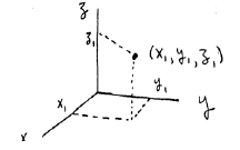
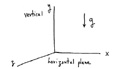
ACCELERATION IN THREE DIMENSIONS

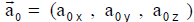
Recall we need three numbers (components) with respect to some
reference point to tell where we are in 3D (actually, this defines 3D.)
We also need three numbers (Cartesian or rectangular coordinates)
each for velocity and acceleration in 3D!

For acceleration components of a body given in all three directions, we can treat this as three
separate 1D motions. So, if all three acceleration components are constant in time, we have
similar-looking equations for all three x, y, z coordinates (which give us the displacements in all
three dimensions). See below where we just add subscripts to distinguish the three numbers
we need for velocity and acceleration

CONSTANT ACCELERATION FORMULAS FOR ALL COORDINATES

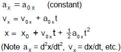
The above must have come from some constant which implies we have constant
acceleration where every acceleration component is constant.

THE CONSTANT SURFACE GRAVITY ACCELERATION g
Ubiquitous Example Of Constant Acceleration

At the surface of the earth (and we’ll learn where we get this in Chapter 4), gravity
vertically exerts a constant force—so that there is a “downward” constant acceleration.

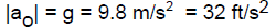
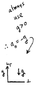
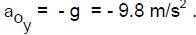
(We use g > 0 always and we put in explicitly any negative sign that may be
needed in front of g. So, for example, if the y axis is positive upward and gravity is
downward:

Added note: Most texts use g = 32 ft/s² = 9.8 m/s² = 980 cm/s² in calculations. (For more
accurate numbers, we need to know the latitude – see later discussions on “centripetal” effects.)

In SI, one could even use g = 10 m/s², since it generates only a 2% error!

CONSTANT GRAVITY TRAJECTORY PROBLEMS
Air Friction Neglected for Most of this Course!!!

Quick 1D Trajectory Example:

Note: See Ch 2 for related discussions.

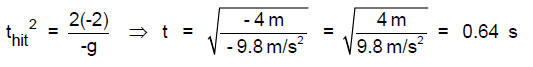
A stone is released from rest, 2 m above ground. How long does it take for the stone to hit the
ground? (The neglect of air friction is not a bad approximation here.)

Solution: With the usual choice of y for the vertical position (with up to be the positive y
direction). You can choose other conventions as long as you stay consistent throughout your
work. In addition, let’s choose the initial time t = 0 where the initial position is and the
initial velocity is Then for the time t_hit that the stone hits the ground,

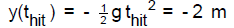
we solve for t (notice how you have to keep track of all the minus signs so that they cancel out
as they must)

********************************************************************************************
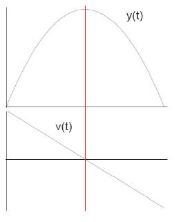
Problem 3-1 To review your old high school stuff, suppose
you throw a ball straight upward with an initial speed of 15 m/s.
You eventually catch the ball when it comes back down. The
plot of its position y(t) is shown on the right and is a good old
parabola symmetric around the vertical red line that goes
through its peak. The velocity v(t) = dy/dt, which is of course
the slope of y(t), is shown in the graph below the y(t) plot.

a) How long will it take to get to the maximum height?
b) How high (relative to your hand) will the ball go?
c) How long does it take for the ball to fall from its
maximum height back to your hand? Don’t use
symmetry but check your answer against (a). (For
posterity, we prove the symmetry below; but don’t use
it, pretty please!)
d) What will the speed of the ball be when you later catch
it in your hand? Again, don’t use symmetry but
compare your answer to the initial value .

********************************************************************************************
Symmetry Proof: We can prove this fast since we can put our origin, y=0, t=0, at the peak
so that times on the left of the red line are negative. Then, if we can show y(-t) = +y(t) and v(-t)
= - v(t), for any t, we are done! With y=0, t=0 at the peak, then , and
we have y(t) = -1/2gt² and v(t) = -g t . We immediately see y(-t) = y(+t) and v(-t) = - v(+t) .
Q.E.D. (You already knew this for a parabola from math class so ... never mind! - Gilda Radner)

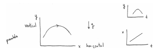
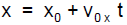
2D Trajectory Formulas:
Now we add the horizontal directions to our motion in constant gravity in the negative y
(vertical) direction. Therefore, , in addition to in our boxed
equations of p. 3-1. The corresponding picture is

It is important to note that these three coordinates evolve independent of each
other and we’ll see the implications of that over and over.

Why do we just talk about 2D instead of 3D in much of our trajectory stuff? Well, motion
will be in planes (the directions of the initial velocity and gravity determine a plane to
which the motion will be restricted, so choose the x-y plane for convenience to be that
plane and we will therefore only need x-y plots from now on!!

We are often interested in y(x) plots to go along with our old time plots, y(t) and x(t).
The general kinds of plots we get are parabolas for y(t) and straight lines for x(t). (This
means that y is a quadratic function of t and x is a linear function of t.) We also get
parabolas for y(x) because if we take the relation x(t) and then solve it for t in terms of x ,
and then substitute it into y(t), we get y as a quadratic function of x. The various plots
look like :

The general formulas are

1) For zero acceleration in the x direction, we have the linear relation for x and v_x is constant:

and = constant

2) For acceleration –g in the y direction, we have the quadratic relation for y
and the linear relation for v_y :

Simple 2D Trajectory Example: A stone is thrown horizontally with a speed 3.0 m/s
from the edge of a cliff

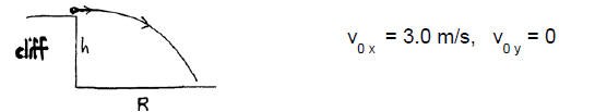
Choose the initial position of stone to be x₀ = y₀ = 0 at t₀ = 0. Suppose it hits the
ground at t = 2.0s. Where does it hit? That is, what are the h and R shown in the
figure?

Vertically:

Horizontally:

Notice the irrelevance of v_{0 x} (and x) to the h calculation here! You’ll think about this
kind of thing in the following problem.

********************************************************************************************

Problem 3-2

a) Suppose someone in 2010 shoots marbles horizontally off of one of the tallest
buildings in the world (in Hong Kong) that is presently under construction and will
be 490 m high. She will shoot one marble at a horizontal velocity of 10 m/s and a
second one at a horizontal speed of 20 m/s. Calculate the time it takes each
marble to reach the ground, neglecting as always air drag. Discuss any
interesting aspect you see in your answers (we don’t mean the terrible possibility
that someone might get hit!).

b) Suppose now she releases two marbles off the first building at the same time.
One of the marbles is shot off horizontally with a speed of 10 m/s. The other
marble is dropped straight down, without an initial velocity. Use graph paper to
plot the y(x) graphs of the two trajectories. Draw them on the same coordinate
system (i.e., side-by-side). Also indicate on each trajectory with big black dots
(or purple ones, maybe) the instantaneous position of the marbles at every
second during the fall. Discuss any interesting aspect you see in the drawing of
the dots.

Note: In (b) you’ve just drawn a “strobe picture” of motion—see the Appendix!
********************************************************************************************

APPENDIX: STROBE FLASH PICTURES
“Particle Motion Diagrams”

Let’s extend what we did in part (b) of the previous homework problem by drawing more “motion
snapshots”—or strobe diagrams. Drawings of objects changing position for a sequence of
equally-spaced time intervals can be useful for understanding the connections among position,
velocity, and acceleration.

Consider two cars A and B, where A starts out at a time t₁ ahead of B, and the two cars travel at
constant velocities that are different from each other. Let’s represent the cars with big black
dots, so that you can easily see how far each car has gone during each time interval:

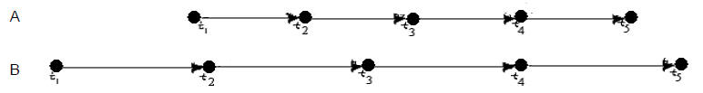
The positions of the two cars at times t₁, t₂, t₃ ... are shown so that, for example, A is in front of B
at time t₁ but behind at t₅. The time intervals between the flashes for each car are chosen to be
equal, and the arrows drawn between each successive position represents the change in the
car’s position. We see that for constant time intervals, the length of the arrow connecting
each strobe flash position is proportional to its velocity. So we can compare the 1D velocities in
such a picture simply by comparing the lengths of the arrows!

Now consider a car that starts from rest and accelerates to a steady speed for a short distance,
then brakes to a halt. Its strobe diagram looks like

Again, since the strobe flashes are at equal times, the spacing (the length of any arrow)
between any two dots indicates the relative speed between flashes. We can also look at the
difference in the lengths of any two successive arrows to approximate the acceleration at that
time. For example, if an arrow is longer than the arrow just preceding it, we have an increase in
speed over the two intervals. A shortening of an arrow compared to the previous arrow indicates
a proportional decrease in speed.

******************************************

Problem 3-3 The figure shows six sequential frames, 1-6, for the motion diagram of two moving
cars, A and B.

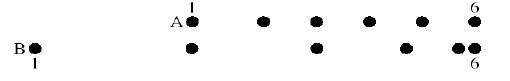
(a) Do the two cars ever have the same position at the same instant of time? If so, identify the
frame number(s).
(b) Do the two cars ever have the same average velocity over the same interval in time? If so,
identify the frame number(s).
******************************************