Economic Optimization
I. Functions and Economic Relationships
Univariate Functions
y=f(x)
X is a variable; it changes its value.
Y is a function of X; If X changes, Y changes as well.
f(...) is a general representation of functional forms (linear, quadratic,
logarithmic , etc.).
Y is a univariate function; this means that Y is a function of only one
variable.
Examples:
a). 
Y is a quadratic function of X.
a, b, c are constants ( parameters or coefficients ); they are numbers and they do
not change their values.

b). y=bx+c
Y is a linear function of X.
b, c are constants; they are numbers, they do not change their values.

Multivariate Functions
y=f(x,z)
X and Z are variables; any of them or both can change their values.
Y is a function of X and Z; If X or/and Z changes, Y changes as well.
f(...) is a general representation of functional forms (linear, quadratic,
logarithmic, etc.).
Y is a multivariate function; this means that Y is a function of more than one
variable.
Example:
a). 
1.3. Examples of Economic Relationships
a). 
 is quantity of oranges in pounds per capita
per year,
 is price of oranges in cents per pound.
This formula indicates that quantity of oranges is a function of price of
oranges. However, this formula does not specify:
•a functional form (linear, quadratic, other)
•how much Q changes given a change in P (a magnitude of the change)
•whether this is a positive or a negative response (direction or sign effect).
 a supply or a demand function ???
b).
This formula indicates that the quantity of oranges is a linear function of the
price of oranges. We know:
•the functional form --- linear;
•how exactly the quantity changes given a change in the price
 (a magnitude of the change);
•we know the direction (sign) effect of the change
 a demand function (a negative slope : -0.5).
c).
 is quantity of oranges demanded (consumed)
in pounds per capita,
 is price of oranges in cents per pound;
 is price of apples in cents per pound; Iis
income per capita per year (in $1,000).
This formula indicates that the quantity of oranges demanded is a function of
the price of oranges, price of apples, and income. However, this formula does
not specify:
•a functional form;
•how much Q changes given a change in the prices and/or income (a magnitude of
the change);
•whether this is a positive or a negative response (direction or sign effects ).
d). 
II.Interpretation of the Coefficients (Parameters) in Supply and Demand
Functions
Handout #1
III.Derivatives
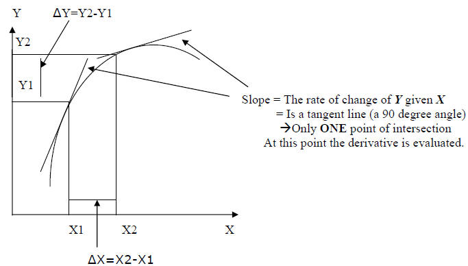
A derivative is a change in a function given a change in the variable.
If y=f(x), then the derivative of Y with respect to X is:

 Marginal value of Y =
Slope of the function

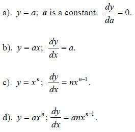
Some important formulas needed to calculate derivatives :


Derivative of a sum is a sum of the derivatives of the
terms.
The derivative of the constant is 0. Therefore, this term is not in the
derivative expression.
IV.Average, Marginal & Total Concepts in Economics
Major Economic Identities
1. Revenue = Price (per unit) *Quantity
2. Cost = Cost (per unit) * Quantity
3. Profit = Revenue – Cost
| Profit = Revenue – Cost | = Price*Quantity – Cost*Quantity |
| = (Price – Cost)*Quantity |
Revenue = Profit + Cost
Cost = Revenue - Profit
General Relationships between the Average and Marginal Values
Suppose AQ and MQ are the average and marginal values, respectively, of some
variables (revenue, cost, profit, etc.).
AQ is decreasing when MQ<AQ,
AQ is increasing when MQ>AQ,
AQ has the first order critical point when MQ=AQ.
If y=f(x), then dY/ dXis the derivative OR a marginal value Y/X is the average
value
Y is the total value.
Example (page 34 of the Text-book)
The total profit function is represented by:

The average profit function is:

The marginal profit (the derivative) is:

Figure 2.5 in the Text-Book (page 35)
V. Economic Optimization
To find the Optimum (Maximum or Minimum) of a function,
Perform the following steps
1.Find the first derivative, and set it to be equal to zero .
2.Solve (1) to find the value(s) of variable(s). These values are the optimums.
3.To determine whether a particular value (optimum) is a maximum or a minimum,
find the second derivative.
The second derivative is the first derivative of the first derivative expression
found in (1).
4.Evaluate the second derivative at each of the variable values found in (2).
5.If the second derivative is negative, then the point is a relative maximum; if
the second derivative is positive, than the point is a relative minimum.
For a relative maximum: dY/dX=0 and
For a relative minimum: dY/dX=0and 
When you are asked to take a derivative, in many cases you will have to solve a
quadratic equation. The general form of these equations is :

To find the roots of the equation , use the formulas:

| Prev | Next |