Matrix Concepts and MATLAB Matrix Computations

(Engineering Analysis and MATLAB 7 - Chapter 5 p 92-100, Chapter 6 p 142-145, Chapter 9 p 247-260,
Chapter 10 276-278)

MATLAB Linear Interpolation (Engineering Analysis and MATLAB 7 - Chapter 11 p. 291-299)

Topics:
1. Matrix concepts - review some old ones and introduce some new ones
2. Introduce solving systems of linear equations using MATLAB matrix computations
3. Concept of interpolation and how it is handled in MATLAB

Notes:

-We have spent the first four weeks developing engineering problem solving methods , building a
foundation of programming concepts, and developing your foundation of MATLAB skills

- I have spoken often about how MATLAB is built for matrix operations but we have mostly used it in
calculations involving scalars (single value 1x1 array) and vectors (1 x n or n x 1 array), both
considered 1 dimensional arrays

Lets review what we have learned about the MATLAB matrices we have been using during our
programming thus far:

Chapters 5, 6, and 8

- User generated arrays:

o X= 4 is a scalar (1 x 1 array)
o Row vector x=[2,4,6,8] Column vector y=[1;2;3;4]
o x(1) returns?
o x = [2,4,6,8;10,12,14,16;18,20,22,24] is a 4x3 matrix



indices are



o What value is x(5) =?
o See example below
>> x=[2,4,6,8;10,12,14,16;18,20,22,24]

>> x(5) %can get a value from a particular location



>> x(5)=100 % can replace a value with another number

o How about in an equation?

>> y= x(5)*500
y =
50000

o Can use this in outputting data as well

> fprintf ('this example should output x(5) %4.3f',x(5))
this example should output x(5) 100.000

Time savers and commands

o Evenly spaced vector time saver B=1:5 or B=[1:5] (colon separator)
o If you want them spaced a certain way time = 0:2:100 gives a vector between 0 and 100
in steps of 2
o linspace - used if you want a certain amount of elements between 2 numbers

>> r=linspace(0,14,5)

-But when do we use 2 dimensional arrays or matrices? They can store data in rows and columns.
These matrices play an important role in linear algebra and are used in science and engineering to
describe many physical quantities.

Consider an electrical circuit (p 253):

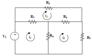
- Based on two basic electrical facts:

Σ voltages around circuit = 0 and V = iR

- And assuming we know the voltage (V) and all of the resistances (R), we can solve for all of the
values of the current by evaluating each loop - we will have 3 equations and 3 unknowns. (See
details p 258)

Can you see the matrix here? How about 3 arrays? We can solve these simultaneously for   using
matrices in various ways.

-Consider a simpler system of equations:

This system of equations can be written as AX=B. Simplify by replacing x with with and z
with

Replacing the coefficients with A and B yields:

can be written in matrix form as:

or in matrix notation as AX=B.

Replacing the numerical coefficients yields:

A = the 3x3 matrix, X = the column vector , and B = the column vector 10,5,1

MATLAB can solve this for and ! We will discuss this in lab!

Chapter 9 Mathematical Operations with Arrays - we need to be familiar with these

These operations between Arrays can be different than standard arithmetic operations . Scalars can be
added, subtracted, multiplied and divided into matrices according to standard operations

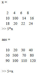
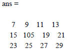
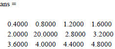
>> 5/x
??? Error using ==> mrdivide
Matrix dimensions must agree.

>> x/5

• Matrix addition and subtraction : Add or subtract the corresponding elements of two arrays of
identical size, e.g.,

- Matrix addition is commutative, i.e., A+ B=B+ A

- When scalar is added or subtracted to an array , it is added to or subtracted from each element in
the array

• Array multiplication: Only possible when the # of columns in the first array is equal to # of rows
in second array, e.g., when A*B=AB

- Matrix multiplication is not commutative, i.e., A*B≠B*A

- Resulting matrix has same # of rows as first matrix and same # of columns as second matrix

- When an array is multiplied by a scalar or number (or a 1×1 matrix), each element in the array
is multiplied by that quantity (multiplication of a matrix with a scalar is a commutative
property )

- Two vectors can be multiplied only if both have same # of elements and one is row and the
other column vector; the result is a 1×1 matrix or scalar; can use built-in Matlab function dot
(a, b) to calculate the product of vectors a and b

- Linear algebra rules of array multiplication can be used to write a system of linear equations as
shown below

can be written in matrix form as

or in matrix notation as AX=B

• Array division: More complicated than multiplication

Inverse of matrix: Matrix B is an inverse of matrix A, if when multiplied, they yield an
identity matrix, i.e., BA=AB=I

- Only applicable to square matrices

- Inverse of A (A^-1) in MATLAB is written as A^-1 or inv(A)

- Only square matrices with non- zero determinants have inverses

****Left division (\): When B and X are both column vectors and A an array, where AX=B,
X=A\B

- Left division is used to solve linear equations

Right division (/): When X and D are row vectors and C an array, where XC=D, X=D/C
- Also used to solve linear equations

• Because of the rules of linear algebra and arrays we have to use the “period” to conduct
element-by-element operations: Addition and subtraction are already element by element.
However, multiplication and division may be both between arrays (discussed earlier) and between
elements.

Arithmetic operators are: a.*b, a./b, a.\b, and a.^b (this can trick you when using scalars)

- Note that the period always precedes the arithmetic operator

- Do NOT have to use the dot (.) before addition and subtraction signs or when multiplying
or diving by a scalar (it will still work though)

- Built-in functions for analyzing arrays: sum, mean, max, min, det, inv, cross, and dot are
also useful .

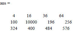
Example of raising a matrix to a power

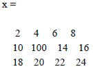
>> x^2
??? Error using ==> mpower
Matrix must be square.

>> x.^2

In lab today - will discuss solving simultaneous equations using matrix operations, the
SOLVE Function, and interpolation