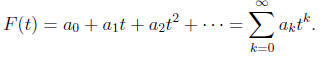
Moment Generating Functions

1 Generating Functions

1.1 The ordinary generating function

We define the ordinary generating function of a sequence. This is by far the most
common type of generating function and the adjective “ordinary” is usually not used.
But we will need a different type of generating function below (the exponential gen -
erating function) so we have added the adjective “ordinary” for this first type of
generating functio.

Definition 1. Suppose that a₀, a₁, . . . is a sequence (either infinite or finite) of real
numbers. Then the ordinary generating function F(t) of the sequence is the power
series

We give two examples , one finite and one infinite.

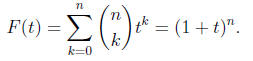
Example 2 (A finite sequence). Fix a positive integer n. Then suppose the se-
quence is given by

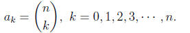
Then the ordinary generating function F(t) is (the binomial theorem ) given by

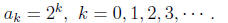
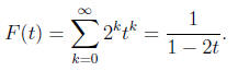
Example 3 (An infinite sequence). Suppose the sequence is given by

Then the ordinary generating function F(t) is (an infinite geometric series) given by

1.1.1 Recovering the sequence from the ordinary generating function
Problem Suppose we were given the function F(t) in either of the two above ex-
amples. How could we recover the original sequence? Here is the general formula.

Theorem 4 (Taylor’s formula). Suppose F(t) is the ordinary generating function
of the sequence a₀, a_1, a₂ · · · . Then the following formula holds

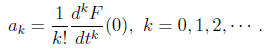
Check this out for k = 0, 1, 2 and the two examples above.

1.2 The exponential generating function

In order to get rid of the factor of k ! (and for many other reasons) it is useful to
introduce the following variant of the (ordinary) generating function.

Definition 5. Suppose again that a₀, a_1, . . . is a sequence (either infinite or finite) of
real numbers . Then the exponential generating function E(t) of the sequence is the
power series

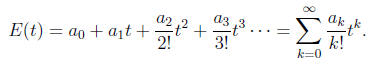
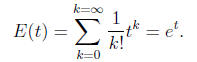
Example 6 (The exponential function). Suppose the sequence is the constant
sequence given by

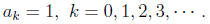
Then the exponential generating function E(t) is (the power series expansion of e^t)
given by

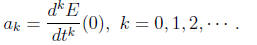
1.2.1 Recovering the sequence from the exponential generating function

The rule for recovering the sequence from the exponential generating is simpler.

Theorem 7. Suppose E(t) is the exponential generating function of the sequence
{a_k : k = 0, 1, 2, · · · }. Then the following formula holds

2 The sequence of moments of a random variable

In this section we discuss a very important sequence (the sequence of moments)
associated to a random variable X . In many cases (and most of the cases that
will concern us in Stat 400 and Stat 401) this sequence determines the probability
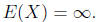
distribution of X. However the moments of X may not exist.

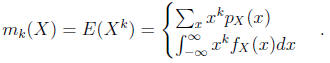
Definition 8. Let X be a random variable. We define the k-th moment m_k(X)
(assuming the definition makes sense, see below) by the formula

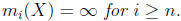
Remark 9 (Moments may not exist). The problem is that the sum or integral
in the definition might not converge. As we said this won’t happen for any of the
examples we will be concerned with. We will give some examples where moments fail
to exist.

Example 10.
Suppose X has t-distribution with n-degrees of freedom. Then
exist but In the special case that n = 1 we have

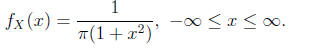
This distribution is called the “Cauchy distribution” and we have

We will ignore the problem that moments might not exist from now on.
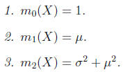
We can calculate the first three moments.

Proposition 11.

Proof. We will prove only (3). The first two are definitions. The “shortcut formula”
for variance says

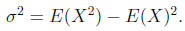
Bring the second term on the right -hand side over to the left-hand side and then
replace E(X) by μ.

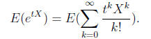
3 The moment generating function of a random variable

In this section we define the moment generating function M(t) of a random variable
and give its key properties. We start with

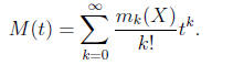
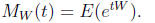
Definition 12. The moment generating function M(t) of a random variable X is the
exponential generating function of its sequence of moments. In formulas we have

Before stating and proving the next key formula we remind you that any function
of a random variable is a random variable. So if we take the family of functions
(depending on the parameter t) defined by g_t(x) = e^tx then we get a family of random
variables e^tX. Then if we take the expectation (one value of t at a time) of the family
e^tX then we get a function of t. Amazingly this function is the moment-generating
function M(t). Put very roughly, the E in the above formula operates on X and t
just goes along for the ride.

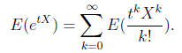
Theorem 13.

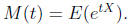
Thus we have

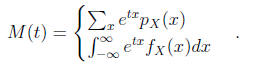
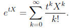
Proof. By the series expansion of the function e^tx we have an equality of random
variables

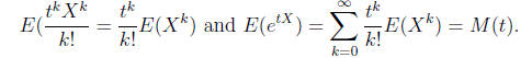
Now take the expectation of both sides to get

Now we use that E of a sum is the sum of the E′s. Unfortunately the right-hand
side isn’t an actual sum, it is an infinite series and we should be careful. However we
won’t worry about this and we get

Now E operates on X and t is a constant as far as E is concerned so we get

Remark 14. We didn’t give a completely rigorous proof above but it shows the main
ideas and is well worth trying to understand, especially because the main property of
M (t), see Theorem (17) follows immediately from the Theorem (13).

4 The moment generating function for the sum of
two independent random variables

In this section we will state two theorems which are both very important. The one we
will be using all the time is the second theorem (the product formula for the moment
generating function of the sum of two independent random variables). However this
formula would not be of any use if we didn’t know that the moment generating
function determines the probability distribution.

Theorem 15. Suppose two random variables X and Y have the same moment-
generating function M(t) (and the series for M(t) converges for some nonzero value
of t). Then X and Y have the same probability distribution.

Remark 16. For Stat 400 and Stat 401, the technical condition in parentheses in
the theorem can be ignored. However it is good to remember that different probability
distributions can have the same moment generating function - even though we won’t
run into them in these courses.

Now here is the theorem we will use all the time in Stat 401. Don’t forget that the
sum of two random variables is a random variable. In Stat 401 we will need results
like “the sum of independent normal random variables is normal” or the “sum of
independent binomial random variable with the same p” is binomial. All such results
follow immediately from the next theorem.

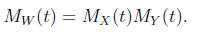
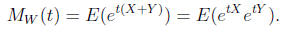
Theorem 17 (The Product Formula). Suppose X and Y are independent random
variables and W = X+Y . Then the moment generating function of W is the product
of the moment generating functions of X and Y

Proof. By Theorem (13) we have

Now plug in W = X + Y to get

Now we use that X and Y are independent. We need two facts. First, if X and Y are
independent and g(x) is any function the the new random variables g(X) and g(Y
are independent. Hence e^tX and e^tY are independent for each t. Second, if U and V
are independent then

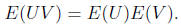
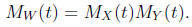
Applying this to the case in hand (one t at a time) we get

Hence:

5 How to combine the Product Formula with your
handout on the basic distributions to find dis-
tributions of sums of independent random vari-
ables

Let’s compute the probability distributions of some sums of independent random
variables. This type of problem is a “good citizen” problem and will appear on
midterms and the final.

Problem 1 Suppose X and Y are independent random variables, that X has Pois-
son distribution with parameter λ = 5 and Y has Poisson distribution with parameter
λ = 7. How is the sum W = X + Y distributed?

Solution Step 1.
Look up the moment generating functions of X and Y in the handout on the basic
probability distributions. We find that if U has Poisson distribution with parameter
λ then

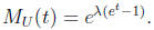
Hence

Step 2.
Apply the Product Formula to obtain

Step 3.(The “recognition problem”)
Find a random variable on your handout that has moment generating function
. Usually (but not always) you don’t have to look very far.

To solve the recognition problem note that we have seen that if U has Poisson
distribution with parameter λ then U has moment generating function . Hence
if we plug in λ = 12 then we get the right formula for the moment generating function
for W. So we recognize that the function is the moment generating function
of a Poisson random variable with parameter λ = 12. Hence X + Y has Poisson
distribution with parameter λ = 5 + 7 = 12. The Poisson parameters add.

Let’s do another example by proving that the sum of independent normal random
variable is normal

Theorem 18. Suppose that X is normal with mean μ₁ and variance and Y is
normal with μ₂ and variance Suppose that X and Y are independent. Then
W = X + Y is normal with mean μ₁ + μ₂ and variance

Proof. From the handout we see that if U is normal with mean μ and variance
then the moment generating function is given by

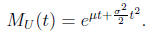
Note that this is the exponential of a quadratic function without constant term, the
coefficient of t is the mean μ and the coefficient of t² is one half the variance .
Hence

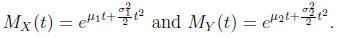
Hence, by the Product Formula we have

Adding exponents in the exponentials we obtain

But we recognize that the last term on the right is the moment generating function
of a normal random variable with meanμ₁ + μ₂ and variance
We do one more example.

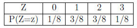
Problem 3, the sum of binomials with the same p is binomial Suppose X
has Bernoulli distribution with p = 1/2 and Y has binomial distribution with n = 2
and p = 1/2. Show in two different ways that X + Y has binomial distribution with
n = 3 and p = 1/2.

First method : without using moment generating functions.
First we find the joint probability mass function in tabular form.
Start with the margins

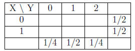
Now fill in the table using that X and Y are independent to get

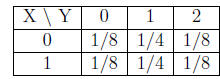
Now compute the probability mass function of Z = X + Y to get

Method 2: using moment generating functions.
From the handout we find

Apply the Product Formula to obtain

Now for the “recognition problem”)
You need to find a random variable on your handout that has moment generating
function (1 − 1/2 + (1/2)e^t)³. Again you don’t have to look very far. To solve the
recognition problem first note (from the handout) that if U has binomial distribution
with parameters n and p then the momment generating function of U is (1−p+pe^t)ⁿ.
Hence if we plug in p = 1/2 and n = 3 we get the right formula for the moment
generating function for Z. So we recognize that the function (1 − 1/2 + (1/2)e^t)³
is the moment generating function of a binomial random variable with parameters
p = 1/2 and n = 3. Hence Z = X + Y has binomial distribution with parameters
p = 1/2 and n = 3.

Remark 19. There is a simple physical explanation for this in terms of coin tossing.
If one person tosses a fair coin once and another tosses a fair coin twice and the two
people add the number of heads they observe the probability distribution they get is the
same as if one of them had tossed a fair coin three times.