Polynomials

Roots

Roots and Divisibility

Lemma 3. Let a be a root of f ∈F[x]. Then (x − a) divides f(x).

Proof.
Write
f = q(x − a) + r
where deg(r) < 1. But then r must be 0, done.

Lemma 4. Any non-zero polynomial f ∈F[x] has at most deg(f) many roots.
Proof.
Use the last lemma and induction on the degree.

Decomposition

So if deg(f) = n and f has n roots we decompose f completely into linear terms :

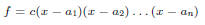
Of course, there may be fewer roots, even over a rich field such as R: f = x^2 + 2 has no
roots.
This problem can be fixed by enlarging R to the field of complex numbers C (the so-called
algebraic completion of R).

More Roots

Note that over arbitrary rings more roots may well exist.
For example over R = Z₁₅ the equation x^2 − 4 = 0 has four roots: {2, 7, 8, 13}.
But of course

Exercise 6. Using the Chinese Remainder Theorem explain why there are four roots in
the example above. Can you generalize?

Point-Value Represenation

The fact that a non- zero polynomial of degree n can have at most n roots can be used to
show that the interpolating polynomial

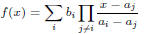
is unique: suppose g is another interpolating polynomial so that g(a_i) = b_i.
Then f − g has n + 1 roots and so is identically zero.

Hence we have an alternative representation for polynomials: we can give a list of
point-value pairs rather than a list of coefficients.

To the naked eye this proposal may seem absurd: why bother with a representation that
is clearly more complicated? As we well see, there are occasions when point-value is
computationally superior to coefficient list.

Multiplying Polynomials

Suppose we have two univariate polynomials f and g of degree bound n.

Using the brute force algorithm (i.e., literally implementing the definition of multiplication
in we can compute the product ring operations .

Now suppose we are dealing with real polynomials. There is a bizarre way to speed up
multiplication:

• Convert f and g into point -value representation where the
support points are carefully chosen.
• Multiply the values pointwise to get h.
• Convert h back to coefficient representation.

FFT

It may seem absurd to spend all the effort to convert between coefficient representation
and point-value representation. Surprisingly, it turns out that the conversions can be
handled in (n log n) steps using a technique called Fast Fourier Transform.

But the pointwise multiplication is linear in n, so the whole algorithm is just (n log n).

Theorem 2. Two real polynomials of degree bound n can be multiplied in (n log n)
steps.

Take a look at CLR for details.

Vandermonde Matrices

Here is another look at conversions between coefficient and point-value representation,
i.e., between evaluation and interpolating.

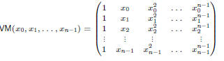
Definition 7. Define the n by n Vandermonde matrix by

Lemma 5.

Evaluation versus Interpolation

It follows that the Vandermonde matrix is invertible iff all the x_i are distinct. Now
consider a polynomial

To evaluate f at points we can use matrix-by-vector multiplication:

But given the values we can obtain the coefficient vector by

Implicit Representation

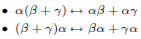
Recall our alternative way of defining polynomials: formal expressions involving ring
elements and the variables using operations plus and times .

We have used this implicit representation in several places already, without any protest
from the audience.

• The expressions encountered
in the root decomposition.
• The description of the determinant of a Vandermonde
matrix
• Using interpolation and evaluation to retrieve the secret in
Shamir’s method.

So?

More precisely, we could consider polynomials to be arbitrary expressions built from
• the variables x₁, . . . , x_n,
• elements in the ground ring,
• addition , subtraction and multiplication.

Obviously we can recover the explicit polynomial (i.e. the coefficient list) from these
explicit representations.

Example 1. Polynomial expands to

We just have to expand (multiply out) to get the “classical form”.
What exactly is meant by “expanding” a polynomial?

Expanding Polynomials

We want to bring a multivariate polynomial into normal form. First
we apply rewrite rules to push multiplication to the bottom of the tree until we have a
sum of products:

Then we collect terms with the same monomial and adjust the coefficent.

Some terms may cancel here (we don’t keep monomials with coefficent 0).

Computationally it is probably best to first sort the terms (rather than trying to do pattern
matching at a distance).

The problem is that it may take exponential time to perform the expansion: there may be
exponentially many terms in the actual polynomial.

Polynomial Identities

A task one encounters frequently in symbolic computation is to check whether two
polynomials are equivalent, i.e., whether an equation between polynomials

holds in the sense that for all

Definition 8. Two polynomials are equivalent if for all
In particular f is identically zero if and 0 are equivalent.

In other words, two polynomials are equivalent iff b

Notation:

Zero Testing

Note that the polynomial identity can be rewritten as

Problem:
How can we check whether a multivariate polynomial is identically zero?

Note: The polynomial may not be given in normal form, but as in the example in a much
shorter, parenthesized form. We want a method that is reasonably fast without having to
expand out the polynomial first.

Using Roots

Assume that the ground ring is a field F.

Suppose f has degree d. As we have seen, in the univariate case there are at most d
roots and d roots determine the polynomial (except for a multiplicative constant).

So we could simply check if the polynomial vanishes at, say, a = 0, 1, 2, . . . , d: f will
vanish on all d + 1 points iff it is identically zero.

Requires only d + 1 evaluations of the polynomial (in any form).

Unfortunately, the roots for multivariate polynomials are a bit more complicated.

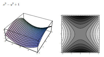
A Quadratic Surface

The Key Lemma

Lemma 6. Let be of degree d and a set of cardinality s.
Then f is not identically zero then f has at most

Proof.
The proof is by induction on n.

The set S here could be anything. For example, over Q we might choose
S = {0, 1, 2, . . . , s − 1}.

Schwartz’s Method

The main application of the lemma is to give a probabilistic algorithm to check whether a
polynomial is zero.

Suppose f is not identically zero and has degree d.
Choose a point uniformly at random and evaluate Then

So by selecting S of cardinality 2d the error probability is 1/2.
Note that the number of variables plays no role in the error bound.

A Real Algorithm

To lower the error bound, we repeat the basic step k times.

// is f identically zero ?
do k times
pick a uniformly at random in Sˆn
if( f(a) != 0 )
return false;
od
return true;

Note that the answer false is always correct.
Answer true is correct with error bound " provided that

Certainty

With more work we can make sure the f really vanishes.

Corollary 1. Let be of degree d and a set of cardinality
s > d. If f vanishes on then f is identically zero.

But note that for finite fields we may not be able to select a set of cardinality higher than
d.

Recall the example over Z₂: in this case we can essentially only choose S = Z₂, so only
degree 1 polynomials can be tackled by the lemma.

That’s fine for univariate polynomials (since any monomial xⁱ simplifies to x) but useless
for multivariate polynomials.

Application

Recall that a perfect matching in a bipartite graph is a subset M of the edges such that
the edges do not overlap and every vertex is incident upon one edge in M.

There is a polynomial time algorithm to check whether a perfect matching exists, but
using Schwartz’s Lemma one obtains a faster and less complicated algorithm.

Suppose the vertices are partitioned into u_i and v_i, i = 1, . . . , n .

Define a n × n matrix A by

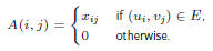
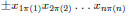
Note that the determinant of A is a polynomial whose non-zero terms look like

Testing Perfect Matchings

Proposition 4. The graph has a perfect matching iff the determinant of A is not
identically zero.

Proof.
If the graph has no perfect matching then all the terms in the determinant are 0 (they all
involve at least one non-edge).

But if the graph has a perfect matching it must have the form
where π is a permutation.

But then the determinant cannot be 0 since the corresponding monomial cannot be
cancelled out.