Quadratics
The objective functions used in linear least -squares and
regularized least-squares are multidimensional
quadratics. We now analyze multidimensional quadratics further . We will see many
more
uses of quadratics further in the course, particularly when dealing with
Gaussian distributions .
The general form of a one-dimensional quadratic is given by:


This can also be written in a slightly different way (called standard form):


where  . These two forms are equivalent, and
it is
easy to go back and forth between them (e.g., given a, b, c, what are
 ?). In the latter
form, it is easy to visualize the shape of the curve: it is a bowl, with minimum
(or maximum) at
b, and the “width” of the bowl is determined by the magnitude of a, the sign of
a tells us which
direction the bowl points (a positive means a convex bowl, a negative means a
concave bowl), and
c tells us how high or low the bowl goes (at x = b). We will now generalize
these intuitions for
higher-dimensional quadratics.
The general form for a 2D quadratic function is:


and, for an N-D quadratic, it is:


Note that there are three sets of terms: the quadratic terms
 , the linear terms

and the constant term  .
.
Dealing with these summations is rather cumbersome. We can simplify things by
using matrixvector
notation. Let  . Then we can write a
quadratic as:


where


You should verify for yourself that these different forms
are equivalent: by multiplying out all the
elements of f(x), either in the 2D case or, using summations, the general N − D
case.
For many manipulations we will want to do later, it is helpful for A to be
symmetric, i.e., to
have  . In fact, it should be clear that these
off-diagonal entries are redundant. So, if we
are a given a quadratic for which A is asymmetric, we can symmetrize it as:


and use  instead. You should confirm for
yourself that this is equivalent to the
original quadratic.
As before, we can convert the quadratic to a form that leads to clearer
interpretation:


where  , assuming that A-1 exists. Note the
similarity here to the
1-D case. As before, this function is a bowl-shape in N dimensions, with
curvature specified by
the matrix A, and with a single stationary point μ. However, fully
understanding the shape of
f(x) is a bit more subtle and interesting.
4.1 Optimizing a quadratic
Suppose we wish to find the stationary points (minima or maxima) of a quadratic


The stationary points occur where all values  ,
that is,
  . Let us assume
that A is symmetric (if it is not, then we can symmetrize it as above). This is
a very common form
of cost function (e.g. the log probability of a Gaussian as we will later see).
Due to the linearity of the differentiation operator , we can look at each of the
three terms of
Eq.11 separately. The final (constant) term does not depend on x and so we can
ignore it. Let us
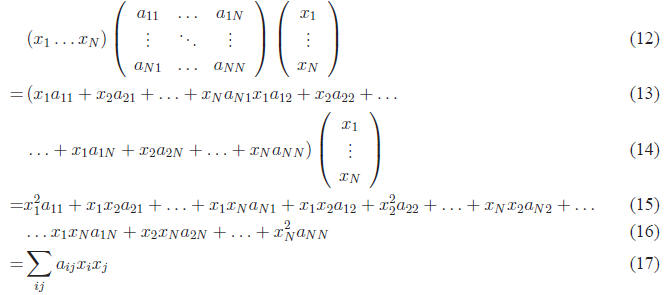
examine the first term. If we write out the individual terms within the
vectors/matrices, we get:

Note that the gradient is a vector of length N, where each
of the terms correspond to  .
.
So in the expression above, for the terms in the gradient corresponding to each
 , we only need
to consider the terms involving  , namely


The gradient then has a very simple form:


We can write a single expression for all of the  using
matrix/vector form:


You should multiply this out for yourself to see that this
corresponds to the individual terms above.
If we assume that A is symmetric, then we have


This is also very helpful rule that you should remember .
The next term in the cost function, bTx,
has an even simpler gradient. Note that this is simply a dot product , and the
result is a scalar:


Only one term corresponds to each
![]() and so
and so
 . We can again express this in matrix/
vector form:


This is another helpful rule that you will encounter again. If we use both of
the expressions we
have just derived, and set the gradient of the cost function to zero , we get:


The optimum is given by the solution to this system of equations:


In the case of scalar x, this reduces to x = −b/2a. For linear regression: A =
XXT and b =
−2XyT . As an exercise, convince yourself that this is true.
| Prev | Next |