Systems of Linear Equations

Now let us eliminate the appearance of x from the third equation.
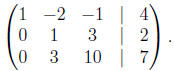
To do this add the first equation to the third equation.

x - 2y - z = 4
y + 3z = 2
3y + 10z = 7.

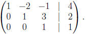
The next step is to eliminate y from the third equation by using the
second equation. To do this, take the second equation, multiply it by
-3 and add it to the third equation,

x - 2y - z = 4
y + 3z = 2
z = 1.

This completes the elimination step. Notice the characteristic upside
down staircase shape of the equations. Now we do backwards substi-
tution. Since the last equation does not involve either x or y, we read
o the value for z from the last equation, to get z = 1. Now take this
value for z and use the second equation, which does not involve x to
solve for y ,

y + 3 = 2.

This gives y = -1. Finally substitute the values for x and y to deter-
mine x,

x + 2 - 1 = 4,

to get x = 3. The solution is (x, y, z) = (3,-1, 1) ∈ R³. It is easy to
check that this is indeed a solution. Strictly speaking we should also
check that there are no other solutions. We will come to this point
later.

Let us introduce some notation, which for the time being we will
think of as just being a convenience. Instead of carrying around the
variables x , y, z etc, let us just put the information into a table. We
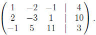
represent the system

x - 2y - z = 4
2x - 3y + z = 10
-x + 5y + 11z = 3.

by the augmented matrix

The coefficient matrix is

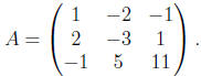
A is a matrix with three rows and three columns, denoted 3× 3. Note
that the rows represent equations and the columns variables. Let

b is also known as a column vector. Clearly b, as a matrix, is 3×1.
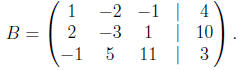
Then the augmented matrix is formed from the two matrices A and b



If we let

then we may also write down the system of equations very compactly
as

Av = b.

It is possible to undefirstand the previous method of solving linear equa-
tions in terms of the augmented matrix only. We start with,

The first step is to take the first row, multiply it by -2 and add it
to the second row,

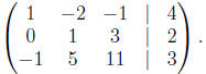
This puts a zero in the second row, first column. The next step is to
take the first row, multiply it by 1 and add it to the third row,

This puts a zero in the third row, first column. The next step is to
take the second row, multiply it by -3 and add it to the third row,

This puts a zero in the third row, second column. At this stage, we
think of this augmented matrix as representing a system of equations
and use the old method of back substitution to solve this system.

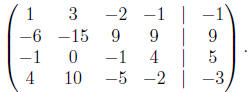
Let us look at a slightly more complicated example. Suppose that
we start with a system of four equations in four unknowns ,

x + 3y - 2z - w = -1
-6x - 15y + 9z + 9w = 9
-x - z + 4w = 5
4x + 10y - 5z - 2w = -3.

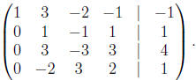
We first replace this by the augmented matrix,

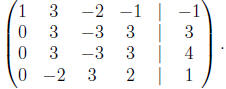
The first step is to use the one in the first row, first column to eliminate
the -6, -1 and 4 from the first column. To do this we add 6, 1, -4
times the first row to the second, third and fourth row, to get

The next step is to multiply the second row by 1/3 to get a one in the
second row, second column,

Now we eliminate the 3 and the -2 in the second column. To do this
we add -3 and 2 times the second row to the third and fourth row,

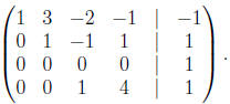
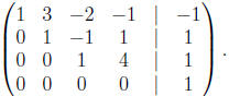
The next step is to get a one in the third row, third column. We cannot
do this by rescaling the third row. We can do it by swapping the third
and fourth rows,

Consider what happens when we try to solve the resulting linear equa -
tions by back substitution. The last equation reads

0x + 0y + 0z + 0w = 2.

There are no values for x, y, z and w which work. The original system
has no solutions. Now suppose we start with the system

x + 3y - 2z - w = -1
-6x - 15y + 9z + 9w = 9
-x - z + 4w = 4
4x + 10y - 5z - 2w = -5.

The only thing we have changed is 5 to 4 = 5 - 1. If we follow the
same steps as before, we get down to the same matrix, except that the
last entry is 0 = 1-1 (remember at some point we swapped two rows)

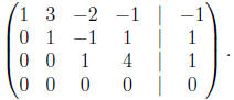
The last equation

0x + 0y + 0z + 0w = 0,

places no restriction on x, y, z and w. The previous equation reads,

z + 4w = 1.

Using this equation, we can solve for z in terms of w, to get z = 1-4w.
We can use this value for z in the second equation to determine y in
terms of w,

y - (1 - 4w) + w = 1,

to get y = 2 - 5w. Finally, we can use this value for y and z in the
first equation to solve for x,

x + 3(2 - 5w) - 2(1 - 4w) - w = -1,

to get

x = -5 - 8w.

We get the family of solutions,

(x, y, z, w) = (-5 + 8w, 2 - 5w, 1 - 4w,w).

Note that no matter the value of w, we get a solution for the original
system of linear equations . For example if we pick w = 0, we get the
solution

(x, y, z, w) = (-5, 2, 1, 0),

but if we choose the value w = 1, we get the solution

(x, y, z, w) = (3,-3,-3, 1).

In particular this system has infinitely many solutions. As before the
reason for this is because the original system of equations was not
independent. In fact even the first three equations are not independent.
We can think of this as being the same thing as the first three rows are
not independent. The third row minus four times the first row is the
same as the second row plus the first row (we can see this by following
the steps of the Gaussian elimination). This is the same as saying the
third row is equal to the second row plus three times the first row. It is
then automatic that any solution to the first equation and the second
equations is a solution to the third equation. Note also that we can
represent the solutions in a slightly different way ,

(x, y, z, w) = (-5, 2, 1, 0) + w(8,-5,-4, 1).