Numerical Methods Lecture 2 Simultaneous Equations

Topics: matrix operations
solving systems of equations

Matrix operations:

Mathcad is designed to be a tool for quick and easy manipulation of matrix forms of data. We’ve seen the
matrix before as a 2-D array. That is, many pieces of information are stored under a single name. Different
pieces of information are then retrieved by pointing to different parts of the matrix by row and column
indexes. Here we will learn some basic matrix operations: Adding and Subtracting , Transpose, Multiplication.

Adding matrices

Add two matrices together is just the addition of each of their respective elements.
If A and B are both matrices of the same dimensions (size), then

C := A + B

produces C, where the i^th row and j^th column are just the addition of the elements (numbers) in the i^th row
and j^th column of A and B

Given: , and
so that the addition is :

The Mathcad commands to perform these matrix assignments and the addition are:



Rule: A, B, and C must all have the same dimensions

Transpose

Transposing a matrix means swapping rows and columns of a matrix. No matrix dimension restrictions
Some examples:

In general



In Mathcad, The transpose is can be keystroked by Ctrl - 1 (the number one )
or you can view the matrix pallet (view -> toolbars -> matrix) and click the  M^T symbol

Multiplication|

Multiplication of matrices is not as simple as addition or subtraction. It is not an element by element multiplication
as you might suspect it would be. Rather, matrix multiplication is the result of the dot products
of rows in one matrix with columns of another. Consider:

C := A * B

matrix multiplication gives the i^th row and k^th column spot in C as the scalar results of the dot product of
the i^th row in A with the k^th column in B. In equation form this looks like:

Let’s break this down in a step-by- step example :

Step 1: Dot Product (a 1-row matrix times a 1-column matrix)
The Dot product is the scalar result of multiplying one row by one column

DOT PRODUCT OF ROW AND COLUMN
Rule:

1) # of elements in the row and column must be the same
2) must be a row times a column, not a column times a row

Step 2: general matrix multiplication is taking a series of dot products
each row in pre-matrix by each column in post-matrix

C(i,k) is the result of the dot product of row i in A with column k in B

Matrix Multiplication Rules:

1) The # of columns in the pre-matrix must equal # of rows in post-matrix
inner matrix dimensions must agree
2) The result of the multiplication will have the outer dimensions
# rows in pre-matrix by # columns in post-matrix

For this example, apply rules

C := A * B

A is nra x nca (# rows in a by # columns in a)
B is nrb x ncb

Rule 1 says:

nca = nrb or else we can’t multiply (can’t take dot products with
different number of terms in row and column)

Rule 2 says:
C will be of size nra x ncb

result C has outer dimensions

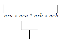
inner dimensions must agree

How to perform matrix multiplication in Mathcad??? Easy

Note: If inner matrix dimensions don’t match, Mathcad can’t perform the operation since it violates the
rules of matrix multiplication, and you’ll get an error that says:

“the number of rows and or columns in these arrays do not match”

example: Let’s try to multiply a 2x3 by another 2x3 (rules say we can’t do this)

Mathcad will tell you:

“the number of rows and or columns in these arrays do not match”

Since the # of columns in A was not equal to # of rows in B, we can’t multiply A * B

IMPORTANT: Another example: Say we create a 1-D vector x with the following:

x:= (3 8 9 5)

Now say we want to square each number in x. It would seem natural to do this:

x^2 =

But Mathcad tells us:

“This Matrix must be square. It should have the same number of rows as
columns”

Note that x^2 = is the same as saying x*x =

Mathcad by default will always interpret any multiplication as a standard dot product type matrix multiplication,
thus we can’t take a dot product of two row vectors, since rules of matrix multiplication are violated
in this case.

The exception to this default assumption in Mathcad is if the vector is a column instead of a row. In that
case, Mathcad will assume you want to square each element in the vector rather that apply standard
matrix multiplication.

If we just want to square the numbers in x, we can do this:

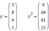
Or we can first convert a row into a column vector using transpose, and then square
Try this out

Practice matrix operations on the following examples.

List the size of the resulting matrix first. then perform the operations by hands. Use Mathcad to confirm
each of your answers.

Solving simultaneous linear equations using Matrix Methods

Now we’ll use matrices to represent sets of algebraic equations . The solution to these sets of equations
can be solved using matrix methods. The simultaneous solution of multiple equations finds its way in to
many common engineering problems. In fact, modern structural engineering analysis techniques are ALL
ABOUT solving systems of equations simultaneously. You’ll see the following material in CES 4141
(structures II) for sure.

• Matrices - an organized way of presenting a set of coupled equations.
• We seek a single unique solution that satisfies all the equations at the same time.
Consider the three coupled linear equations below:

• Coupled because each equation has one or more terms in common with the others, , so
that a change in one of these variables will affect more than one equation.

• Linear because each equation contains only first order terms of . There are no terms
like , or , or , or , etc.

• Using the rules of matrix multiplication, we can represent the above equations in matrix form:

Try multiplying the matrices A and X together, make sure you can get the original equations above.

There are several ways to solve for unknown vector X. Each method involves some manipulations to the
coefficient matrix using algebraic rules, creating a new and equivalent problem in a more easily solvable
form. These manipulations involve the addition of multiples of one row to another.

Adding one row to another results in an equivalent equation, since both sides are equal.

For example, starting with the two equations:

their addition gives:

This addition does not add any new information, but it does present a new form of the old information.

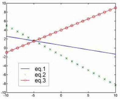
If we plot these 3 equations, the solution is the
place where they intersect. That is, we are seeking
the one pair of X1 and X2 values which lines
along both or the original lines (eq1, eq2).

For only two equations and two unknowns, finding
the solution is trivial substitution . However,
many problems require the solution of many
equations and as many unknowns. If we had 5
equations and 5 unknowns, things get more difficult
to handle with just substitution.

We’ll now look at several ways to systematically
solve a set of simultaneous equations of any size.
First we put the equations in matrix form, then
manipulate the matrix to get a solution.

Gaussian Elimination (method #1):

Consider the three coupled linear equations given earlier. The original form looks like this:

But what if we could recast the same problem to look like this?

This makes life easier, since there is less coupling between equations. In fact, can be solved immediately
using the bottom equation ==> to give . Now the result can be used
to write the middle equation as to get . Finally, the known values
, are used to solve for   in the first equation to get .

This easy solution process is called back-substitution, and is made possible by the lower triangle of zeros
in the coefficient matrix, marked with a dashed triangular box.

Great, it would be nice if the problem looked like Eq. (5), but it actually looks like Eq. (4), so what now?

We can use a series of additions of the 3 equations in Eq. (4) to get it to look like Eq. (5). In a series of
steps just like the above addition of Eqs (1), (2) to get Eq. (3) we’ll reduce the coefficients
to zero, in that order.

KEY: Whatever we do to the l.h.s. of an equation, we do to the r.h.s. so we don’t change the problem.

Let’s rewrite the matrix in Eq. (4) to get one matrix with both A and B in it:
This is called augmenting the matrix.

Step 1) - reduce A(2,1) to zero

New Row 2 = (Row 1)(-2/3) + (Row 2)
Row 1 is called pivot row for this step. Some multiple of it is added to another equation, but the pivot row
remains unchanged

add

Step 2) - reduce A(3,1) to zero

New Row 3 = (Row1)(-1/3) + (Row 3)
Row 1 is the pivot row again
Expanding this instruction like we did in Eq.(7), the result is

Now we need to reduce A(3,2) to zero. If we added some multiple of Row 1, then A(3,1) would become
non-zero. Instead, we’ll need to add some multiple of Row 2 to Row 3 to get a new Row 3.

Before we go on, let’s consider error reduction...

error reduction - swap Rows 2 and 3

• If there were some numerical error in the computer storage of any coefficient, say the error from
rounding off the -1/3 currently in spot A(2,2), then when we multiply Row 2 by some factor and
add it to Row 3, we also multiply the error by that factor.

• If we can always multiply by some small number (less than 1), we can reduce the propagation of
that round-off error.

• We can enforce this by making sure the lead coefficient (the pivot coefficient) in the pivot row
has the largest absolute value among itself and all the coefficients under it (the coefficients to be
reduced to zero).

• Since it does not matter what order I put the equations in, we will rearrange rows when we find
the current pivot coefficient has a smaller absolute value than those beneath it. In the current
example we have:

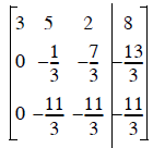
• Row 2 will be the pivot row to eliminate A(3,2), which makes A(2,2) the pivot coefficient. Since
, we’ll swap Rows 2 and 3, and the new pivot coefficient will be largest:

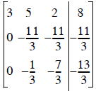
Now we can continue with minimal round-off error propagation

Step 3) - reduce A(3,2) to zero

New Row 3 = (Row 2)(-1/11) + (Row 3)
Row 2 is the pivot row now

Now let’s expand this to its full form with A, X, B in separate matrices

Summary of Gaussian Elimination:

Starting with a problem defined as in Eq. (4), we created some equivalent problem Eq. (5),(12) with the
desired lower triangle of zeros. (12) and (4) are equivalent since all we did was a series of steps where we
added the same thing to both sides of a row.

• Now a little back-substitution (the paragraph following Eq. (5)) gives us

Solution Method 2

The Inverse matrix (matrix version of division):

Let’s take another look at the matrix problem



where we have A, B, and we want to solve for the unknown(s) X. If this were a scalar problem, the
answer is just to divide both sides by A
or . (15)

There is no dividing with matrices, but we can try to find some other matrix (M) to pre-multiply both
sides with such that we’re left with



which says that



What we seek what is called the Identity matrix (denoted I). A square matrix with ones on the diagonal,
and zeros everywhere else. Multiplying any matrix by the Identity matrix (I) is equivalent to multiplying
by one in the scalar world.

TRY IT!! Perform the multiplication in Eq. (18) by hand to see that it’s true.
So Eqs. (16), and (17) say that what we want is some ‘magic’ matrix M such that

or

Back in the scalar world again, we can always get 1 by dividing anything by itself, or multiplying any-
thing by its inverse

So let’s call the matrix we seek, M, the inverse of A, since we want the resulting multiplication to be the

identity matrix. We’ll change the symbol from  M to  A ^-1 to indicate the inverse of A.

What we seek A^-1 is so we can get the solution for from

equivalent to

equivalent to

equivalent to

Gauss-Jordan Elimination - finding the inverse
Gauss-Jordan Elimination I: For the first version of this method, let’s continue where we left off in the
Gaussian elimination example:

where Gaussian elimination is used to get the lower triangle of zeros.
• The idea of Gauss Jordan elimination is to continue the algebra to get an upper triangle of zeros,
until the three equations are completely uncoupled.
• Just as we worked from top to bottom to get zeros for A(2,1), A(3,1), and A(3,2) in that order, we
can start working from the bottom up to make A(2,3), A(1,3), and A(1,2) zero, in that order.
• Just start with the bottom as the pivot row to zero A(2,3), A(1,3), then switch the pivot row to the
second row to make A(1,2) zero.

The three steps to get rid of A(2,3), A(1,3), A(1,2) would be
Step 1) New Row 2 = (Row 3)(-11/6) + (Row 2)
Step 2) New Row 1 = (Row 3)(1) + (Row 1)
Step 3) New Row 1 = (Row 2)(15/11) + (Row 1)
And the result is

We see now that the three equations have been completely uncoupled.
Now if we multiply each row by whatever it takes to make the A coefficient in that row equal to 1, we get

This last bit of making each coefficient equal to one is called normalizing
The solution , , is now shown directly on the right hand side.

Notice that A has been transformed into the identity matrix!

What we have done is built the inverse matrix A^-1  into the right hand side of the equation. So what we
see in Eq. (26) is exactly the result of

Summary of Gauss Jordan Elimination I -

1) Augment coefficient matrix with the solution vector
2) Create lower triangle of zeros
3) Create upper triangle of zeros
4) Normalize the coefficient matrix
5) Values of the unknowns are now in the right hand column

Gauss-Jordan Elimination part II - Finding A^-1 directly

• In the above method, we used Gauss-Jordan elimination, and wound up with the result of A^-1B
on the right hand side.

• We never actually explicitly ‘saw’ A^-1, it was just built in.

We can also used Gauss-Jordan elimination to explicitly compute the inverse of , then multiply
this A^-1 by to get the desired unknowns in  X as in

As you may have noticed, finding A^-1 has nothing to do with what’s in B. Only A is needed to
find A^-1. Let’s look way back at Eq. (6), repeated below

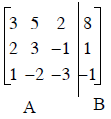A augmented with B. (27)

We augmented the matrix A with B, since we wanted to operate on B.
Now Let’s throw out B and replace it with the identity matrix

If we now use the Gauss-Jordan elimination method to reduce the three left hand columns to the identity
matrix, the result on the right hand side is the inverse of A. We do the exact same steps we did before to
get to Eq. (26). Only this time, instead of tacking on B for the ride, we tack on what starts as I for the
ride. When its all over, the right three columns are A^-1.

Example: we’ll just solve for the inverse of a 2x2
Start with

The steps are:
Step 1) New Row 2 = (Row 1)(-3) + Row 2 .............

finished lower triangle of zeros, now get upper triangle of zeros

Step 2) New Row 1 = (Row 2)(1) + Row 1 ..............

Step 3) Normalize each row: (Row 2)(-1/2)

The result is:

Which means

How can I check to make sure the inverse of is really?????

We know that ,

so let’s try it

This checks out, so we’ve found the inverse

Solving equations using Mathcad

Let’s go back to the original problem in this lecture

Re-written as

Let’s use the built in Mathcad commands to solve the problem defined as:

A*X = B We have the matrix A, and the vector B, find the vector X

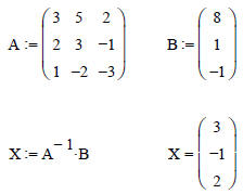
Yep, 13 pages of lecture notes captured in a single Mathcad line

(of course the inverse function contains the Mathcad code to augment the matrix, create the upper and
lower triangles, and normalize)

We can also use a built in function called ‘lsolve’ to calculate the solution t A*X = B

  X := lsolve (A,B)