Solving Error-Locator Polynomials
The only nonlinear step in the decoding of BCH codes is
finding the zeroes of the error -locator
polynomial  . If the number of errors,
 , is not larger than the error correcting
ability of the
, is not larger than the error correcting
ability of the
code, then the degree of is
. Polynomials of small degree can be solved
using various ad
hoc methods. In particular, polynomials over GF(2m) of degree ≤4 can be factored
quickly using
linear methods .
Quadratic polynomials
First we consider an error-locator polynomial of degree 2:
Squaring in GF(2m) is a linear transformation of the vector space GF(2m) over
the scalar field
GF(2). Therefore the equation  can be rewritten as
where x is the unknown m -tuple,  and
and
 are m×m matrices corresponding to
multiplication
are m×m matrices corresponding to
multiplication
by constants and
, S is the m×m matrix over GF(2) that represents squaring,
and 1 is the
m-tuple (1, 0, . . . , 0). Solutions of this system of equations are zeroes of
the error locator polynomial
. The coefficients of the m×m matrix
 involve a matrix
multiplication and
involve a matrix
multiplication and
can be computed in O(m3) bit operations. The rows of the
![]() and
and
![]() matrices can be
obtained
matrices can be
obtained
by shifts with feedback. The squaring matrix S can be precomputed; its rows are
Once A has been found, approximately  bit operations are sufficient to solve the GF(2) system
of linear equations xA = 1. Gaussian elimination uses elementary row operations.
Subtracting
two rows of an m ×m matrix over GF(2) can be performed by XORing two m-bit wide
registers.
Solving xA = 1 can be done in about  row operations. For example, when m = 8, the linear
system can be solved in about 32 clock cycles, compared to 255 evaluations of
in the worst
case for trial and error.
Quadratic polynomials can be solved even faster using the change of variables

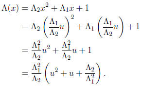
The transformed equation is of the form u2 + u + c = 0 or
U(S + I) = c. It can be solved using
a precomputed pseudo -inverse R of S + I . If U1 = Rc is one zero, then U2 = U1 +
1 is the other
zero, since the sum of the two zeroes is 1. Thus the zeroes of the original
polynomial are
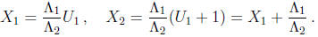
Only half the values of c yield solutions, so we must check that c belongs to the range of S + I .
Another way to solve the simplified quadratic polynomial
is to store the zeroes of the simplified
quadratic polynomials u2 + u + c in a table of 2m entries indexed by the
constant term c. This
approach is feasible if 2m is not too large. The polynomials u2 + u + c have
zeroes in GF(2m) for
exactly half of the elements c in GF(2m). For those values of c for which the
polynomial does not
have zeroes, a dummy entry such as 0 can be stored.
Once the error locators X1 and X2 have been calculated, log tables may be needed
to convert
to symbol error locations  and
and
 .
.
Cubic and quartic polynomials
Cubic polynomials, which arise in triple error correcting codes, can also be
solved using lookup
tables of size 2m. A change of variables of the form x = au + b can transform
the error-locator
polynomial
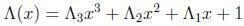
to one of two simplified forms:
 or
or

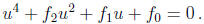
Given a table indexed by c that stores two zeroes U1, U2
of u3 + u + c, the third solution is
 For the other form of reduced polynomial , u3 + c, one zero U1
could be stored
For the other form of reduced polynomial , u3 + c, one zero U1
could be stored
in a table; the other zeroes are  and
and
 , where γ is a cube root of
1. (When m is
, where γ is a cube root of
1. (When m is
odd, every element of GF(2m) has a single cube root, hence u3 +c has one zero of
multiplicity 3.)
Cube roots can also be easily computed using logarithms.
Cubic and quartic polynomials over GF(2m) can also be solved using linear
methods. The
error-locator polynomial of degree 4,

can be reduced by a change of variables of the form x = (au + b)-1 to a polynomial
The zeroes of this polynomial are the solutions of the linear system
where S is the squaring matrix.
Polynomials over GF(2m) can be factored efficiently using Elwyn Berlekamp’s
factoring algorithm
(Bell System Technical Journal, 46:1853-1859, 1967). The running time for
polynomials of
degree n is  for a small exponent c , but the constant factor
 is too large for
many applications.
is too large for
many applications.
Chien search
Using Horner’s method, any polynomial of degree
![]() can be evaluated at a single
point using
can be evaluated at a single
point using ![]()
multiplications and additions. Viktor Pan proved in 1962 that
![]() multiplications
are needed in general.
multiplications
are needed in general.
However, evaluating a polynomial at n points can sometimes be done using much
less than
 operations. For example, the discrete Fourier transform, which consists of
evaluating a polynomial
operations. For example, the discrete Fourier transform, which consists of
evaluating a polynomial
(the input vector) at all n-th roots of 1, can be computed using O(n log n)
multiplications
and additions.
The Chien search is a clever method for solving the error-locator polynomial by
brute force—
we evaluate ![]() for every
i=1,2,...n. The Chien search
evaluates
for every
i=1,2,...n. The Chien search
evaluates  for successive values
of i using ![]() constant multiplications instead of
constant multiplications instead of
![]() general
multiplications. (This is surprising,
general
multiplications. (This is surprising,
because the coefficients  of the error-locator polynomial are not
known in advance.)
of the error-locator polynomial are not
known in advance.)
Furthermore, each evaluation of
![]() takes place in one clock cycle instead of
takes place in one clock cycle instead of
![]() clock cycles—
clock cycles—
without resorting to pipelining techniques.
The key idea of the Chien search is to maintain state variables, Qj for j = 1, .
. . , ![]() , where
, where
 at every time i. Each state variable is easily updated by
multiplication by a constant:
at every time i. Each state variable is easily updated by
multiplication by a constant:
 . The sum of these state variables is
 , so an addition tree is
sufficient to tell
, so an addition tree is
sufficient to tell
when 
A Chien search circuit is shown in the following figure. In this circuit, and in
the modified
Chien search circuits shown later, the memory elements are initialized with the
coefficients of the
error-locator polynomial. When
 , we set
 for
for
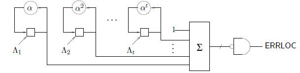
The output signal ERRLOC is true when
 . Since the
zeroes of
. Since the
zeroes of ![]() are the reciprocals
are the reciprocals
of the error-location numbers, ERRLOC is true for those values of i such that
 is
is
an error-location number. Thus as i runs from 1 to n, error locations are
detected from the most
significant symbol down to the least significant symbol.
In the binary case—channel alphabet GF(2)—the ERRLOC signal can be used directly
to
correct the received bit  In the general case, the error pattern Yl must
be computed from the
In the general case, the error pattern Yl must
be computed from the
syndrome equations or by Forney’s algorithm, which is given later in this
handout.
The Chien search is often fast enough because the number of clock cycles it
requires is very
close to the number of information symbols. Thus error correction can be
performed in the time
it takes to compute the syndrome of the next received n-tuple.
A straightforward way to speed up the Chien search is to run two searches in
parallel. The
following circuit is more efficient than two separate copies of the Chien search
engine because the
memory storage elements are shared.
In the above circuit, ERRLOC0 is true when an even error
location is detected, while ERRLOC1
indicates odd error locations. (The additional combinational logic may require a
longer clock
cycle.) The scaler  usually requires more gates than the scaler
 for small
values of j. Thus
for small
values of j. Thus
the complexity of a double -speed Chien search circuit can be further reduced by
factoring the
scalers as

The combinational logic delays of this circuit may be
slightly greater than those of the first
double speed Chien search circuit because the optimized logic for multiplying by
![]() may be faster
may be faster
than the sum of the delays through two
![]() scalers.
scalers.
In practice, the Chien search is often run backwards, using scalers for
 The
The
reverse search locates errors starting with error location 0. When the received
data is already
stored in random access memory, there is no advantage in correcting the symbols
starting with
the most significant symbol 
The error magnitudes Yl , which are given by the Forney algorithm,
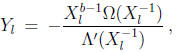
can be computed by a circuit similar to the Chien search
circuit that operates in parallel with the
Chien search. At each time i, the values of
 and
and
 are available, so Yl can be computed
with one division in GF(2m) and one multiplication by
 . Since b is a
constant, successive
. Since b is a
constant, successive
values of  can be computed by multiplication by the scaler
 . The
multiplication
. The
multiplication
by  is not needed when b = 1, which is a minor advantage to using
narrow-sense BCH
is not needed when b = 1, which is a minor advantage to using
narrow-sense BCH
codes.
Although the total number of operations performed is greater than simply
evaluating the polynomials,
the Chien-style circuit uses low -cost scalers and has very simple control logic.
Another
advantage of this approach is that each error magnitude can be computed quickly
after the corresponding
error location is found. For the narrow-sense BCH code, one division operation
is needed
for each corrected error.
| Prev | Next |