Matlab and Numerical Approximation
1 Introductory Remarks
The primary purpose of this course is to provide the
students with the background and
necessary experience (by way of lots of practice) to feel comfortable using the
interactive
software Matlab. Learning any new software presents certain obstacles by way of
needing to
memorize new syntax and becoming familiar with the operating environment. Even
though
Matlab is quite easy to use once you get used to it, we must nevertheless spend
some time
at the beginning to becoming acquainted with the Matlab interface and syntax.
This will be
accomplished in several ways. First the text for the course is the Fourth
Edition of the \Matlab
Primer" by Kermit Sigmon. This book contains a brief but fairly complete
description of the
most elementary aspects of Matlab. Second there are several files in HTML format,
developed
by L. Schovanec and D. Gilliam which cover many topics in the use of Matlab.
2 Xterminal and Matlab Basics
1. To use the xterminals in the lab you must first login.
Directions will be given in class.
2. Next you must open a "command-tool" window or "xterm"
window. Please ask how to
do this if you don't know.
3. The operating system on our computer is UNIX. There
will only be a few cammands
for the operating system that you will need in this class.
4. For example, lets make a subdirectory for your m4330
(or m5344) work, e.g., type mkdir
m4330 . Of course you must then type (return) or (enter) which has the effect of
telling
the operating system to do what was previously typed.
5. Now change to the new subdirectory by typing,
cd m4330 .
6. To run Matlab, at the prompt, simply type matlab and
return and your interactive
matlab session will start.
7. In matlab every object is a complex matrix in which
real entries are displayed as real
and integer as integer.
8. There are several ways to enter a matrix into Matlabs workspace:
(a) You can type in the elements
A=[2 4 5;2 6 3;-1 6 2]
builds a 3×3 matrix. The entries are typed in rows (elements separated by a
space
or a comma) with a semicolon used to declare the beginning of a new row.
(b) You could also generate a matrix using the commands
rand(n) or rand(n,m) to
generate a random n by n or n by m matrix whose elements are normally
distributed
in 0 to 1.
(c) The commands
a=fix(10*rand(5))
b=round(10*rand(5))
generate 5 × 5 matrices with integer entries.
9. If A = [aij ] and B = [bij ] are n £m matrices and C
= [cij] is an m × p matrix, then we
have the following matrix arithmetic operations:
(a) A + B = [aij + bij ] and A - B = [aij - bij ]
(b) A * C = D where D is a n × p matrix with entries
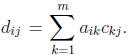 For matrix
multiplication the number of columns of the first matrix must be the same as the
number of rows of the second.
(c) For a number α, the scalar product αA = [αaij]
For example
A=[1 2 5 ;-2 1 4]
B=[4 2 0 ;4 2 -7]
C=[3 6 ;-2 1 ;-4 2]
A+B
A*C
3*A
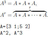
10. The usual rules of positive integer exponents applies for square matrices, A2 = A * A,
11. In general, division of matrices makes no sense. But
for nonsingular square matrices is it
is possible to make an interpretation of matrix division. If A is nonsingular,
then it has
an inverse, i.e., a matrix A-1 satisfying A * A-1 = A-1 * A = I where I is
the identity
matrix with ones on the main diagonal and zeros elsewhere . The identity matrix
plays
the same role as the number 1 does for multiplication A* I = I *A = A. In Matlab
the
identity matrix is given by eye(n) where n is an integer. If A is nonsingular,
then the
inverse in matlab is given by inv(A) or A^(-1). In this case we can think of
division
as B * A-1 just as we do with numbers b ÷ a = b * a-1
for numbers with a ≠ 0.
12. More generally, in this case, you can compute C=A^(-r).
A=[3 1;5 2]
A^(-1), inv(A)
A*A^(-1)
A=[3 1;5 2]
C=A^(-2)
C*A2
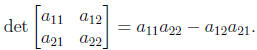
13. A matrix has an inverse if and only if its determinant is not zero. Recall
the determinant
for a square matrix is a number. You can find the definition of the number in most
college
algebra books. In Matlab it is easy to compute determinants using the command
det.
A=[3 1;5 2]
d=det(A)
14. Recall for a 2 × 2 matrix
15. The problem of determining when a square matrix has an inverse is not easy
to answer.
The answer is that precisely the nonsingular matrices have inverses. There are
several
other characterizations of nonsingular given below. We will consider these
properties
with two examples
A=[3 1;5 2]
B=[3 1;6 2]
A matrix A is nonsingular if and only if any one of the following hold:
(a) detA ≠ 0
det(A)
det(B)
(b) The row reduced echelon form of A is the identity
rref(A)
rref(B)
(c) A has an inverse
inv(A)
inv(B)
(d) The only solution of the equation Ax = 0 is x = 0, i.e., the null space is
the zero
vector. The Matlab command \null" computes a basis for the null space. Note It
does not list the zero vector.
null(A)
null(B)
(e) The matrix A has full rank. If A is n × n then the rank of A is n.
rank(A)
rank(B)
16. Since we can do powers , scalar products and sums of matrices we can consider
matrix
polynomials. Here is an example. Suppose A is an n × n matrix, c is a (m+1)
component
row vector, then the matrix polynomial expression


17. Here is an example
A=[3 1;5 2]
c=[-3 2 -1 5]
f=c(4)*A3+c(3)*A2+c(2)*A+c(1)*eye(2)
g=A*(A*(c(4)*A+c(3)*eye(2))+c(2)*eye(2)) +c(1)*eye(2)
%Horner's method or synthetic division
18. Recall that a system of n linear equations in n unknowns has the form
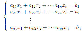
which can also be written in matrix form as
Ax = b
where
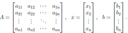
19. A system of equations in this form can be solved in Matlab several different
ways. One
way is to use the \backslash" syntax x = A\b.
| A=[3 1;5 2] | % | setup A |
| b=[2;-9] | % | setup b |
| x=A\b | % | solve Ax=b |
| A*x-b | % | check the result |
20. This system can also be solved by writing the augmented matrix [A b] and
computing
the row reduced echleon form. The last column is the solution.
| A=[3 1;5 2] | % | setup A |
| b=[2;-9] | % | setup b |
| C=[A b] | % | setup augmented matrix |
| rref(C) | % | compute row reduced echleon form |
21. A system of equations in the form xA = c where x and c are row vectors can
be solved
in Matlab using the "forwardslash" syntax x = c/A.
| A=[3 1;5 2] | % | setup A |
| c=[2 -9] % | % | setup c |
| x=c/A % | % | solve xA=c |
| x*A-c % | % | check the result |
22. Additional information and examples can be found in the Matlab Primer and/or
accessing
on- line tutorial files on the webb using netscape.
23. For the assignment below it will be very useful to use the
"diary" command
in Matlab.
The command is used to save input and output into a text file. The syntax diary
on
turns copying on and diary off turns copying off. You can turn diary on and off as
you
please and each time it is turned on the new data will be appended to the
current diary
file in you subdirectory. The diary file can be loaded into a word processor and
edited.
| Prev | Next |