Thank you for visiting our site! You landed on this page because you entered a search term similar to this: how to solve a 2nd order differential equations. We have an extensive database of resources on how to solve a 2nd order differential equations. Below is one of them. If you need further help, please take a look at our software "Algebrator", a software program that can solve any algebra problem you enter!
MA2051 - Ordinary Differential Equations
Matlab - Solve a second-order equation numerically
Start by reading the instructions in wrk4 (or wheun or weuler); just type help wrk4 and focus on the last part of the help. Here is how it goes. To solve
 In vector notation, this system has the form
 ![]() ,
where
,
where
![]()
Now use an editor to create a M-file named frcdsprg.m for this
vector system ![]() :
:
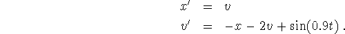
% frcdsprg.m - new version
% x'' + 2x' + x = sin( 0.9 t ) written as the system
%       x' = v,    v' = -x - 2v + sin( 0.9 t)
% y(1) is x, y(2) is v.

function yprime = frcdsprg( t, y )
yprime(1) = y(2);     % x' = v in terms of y's
yprime(2) = -y(1) - 2*y(2) + sin( 0.9*t );    % v' = -x ... in terms of y's
The following sequence of commands will solve this system
with initial conditions x(0) = 1, v(0) = 2
for ![]() .
.
y0 = [1; 2];
[t, y] = wrk4( 'frcdsprg', 0, 30, y0, 0.2 );
The plot that appears is the graph of the approximate solution curve x(t) for
Type [t,y] (without a semicolon). Three columns of numbers will fly by; the first column is t, the second column is y(1) = x(t), and the third column is y(2) = v(t). In the above instructions, notice that you are solving both of the first-order equations at the same time. The initial data is specified in y0 = [1;2], and the time step by 0.2.
The following commands will plot x(t) and v(t) again st t and annotate the plot:
plot(t,y(:,1),'-');                        % plots x(t) with lines
hold on;                                   % holds the old plot
plot(t,y(:,2),'.');                        % plots v(t) with dots
title(' x" + 2 x'' + x = sin(0.9 t)  ');   % adds a title ('' prints as ')
xlabel(' time ');
ylabel(' position and velocity  ');        % label the axes
text(15,1.0,' ...  velocity  ');           % put text at (15,1.0)
text(15,1.5,' --- position ');             % put text at (15,1.5)
Note that y(:,1) refers to the first column of y (which is
x(t)) and y(:,2) refers to the second column of y (which
is ![]() ). To make a new plot, type hold off.
). To make a new plot, type hold off.
The following commands will plot v(t) against x(t) (instead of t), producing a phase plane plot of this nonautonomous system:
plot(y(:,1),y(:,2),'.');                                  % plots x and v
title(' Phase Plane:  x" + 2 x'' + x = sin(0.9 t)   ');   % adds a title
xlabel(' position ');
ylabel(' velocity ');                                     % label the axes
To control the axis limits, type axis( [ -0.75 1 -1 1.5] ); the graph will show ``x'' values from -0.75 to 1 and ``y'' values from - 1 to 1.5. Type help axis for more information.
Alternatively, to get a phase plane plot directly for an autonomous system, type pplane and enter your equations into the text box that appears.
Next: Index
© 1996 .
All rights Reserved. File  November 21, 1996.