solving second order linear difference equation,algebra substitution method calculator,how to solve second order linear nonhomogeneous differential equations,convert mixed fraction to decimal,pre algebra distributive property prentice hall,converting base 2 fraction to decimal fraction,adding subtracting multiplying dividing integers,dividing fractions and mix numbers cheat problem solver,solving second order homogeneous differential equations,solving basic algebra equations homework word problem,rules for adding variables in a square root,error 13 dimension on a ti 86 graphing calculator solving linear equations,Matlab solve second order differential equations,quadratic equation graph hyperbola,Adding, subtracting, multiplying and dividing Integer worksheets,factoring polynomials with a cubed term, tutorial,linear equation in two variables subject to linear constraint inequalities,finding the least common denominator for two rational expressions,slow steps balancing chemical equations with least common multiples,pre algebra definitions open algebraic expression,slow steps for balancing chemical equations with least common multiples,Like Terms Simplifying Algebraic Expressions Junior High,convert decimal to square root fraction,value for variable expression radicals roots,Quadratic Equation Calculator factor,TI- 83 ,84 graphing calculator step by step of how to use to find slope of lines graphing calculator,worksheets on add subtract multiply divide fractions,how to solve multivariable algebra equation with fractions,how do you divide and times add subtract integers worksheet,math poems with the words, prime numbers, common multiples,common factors,combining like terms in algebraic expressions worksheets,prealgebra solving equations by multiplying and dividing worksheet,simplifying exponents and square root calculator,multiply and divide rational expressions calculator,Like Terms Simplifying Algebraic Expressions Activities Lessons,adding subtracting dividing multiplying integers games,Simplifying a sum of radical expressions calculator,converting base 8 to decimal calculator,adding and subtracting positive and negative integers free worksheets,practice worksheets on adding, subtracting,multiplying,and dividing decimals. for 6th grade,What are sqaure root method of Quadratic Equations?,greatest common factor for three number with variables,solving nonlinear differential equations matlab,Java method Convert Decimal Numbers to time,solving NONLINEAR simultaneous equATIONS USING MATLAB,ti-83 plus solving systems of linear equations in three variables,solving quadratic equations completing the square,integers adding, subtracting, multiplying, dividing worksheet,how do you do the square root on the TI-83 plus graphic calculator?,multiple choice exponents algebra powerpoint rules,solving absolute value and radical equations using restrictions,7th grade level variables and equations explanations Equations Substitution variables,Uniqueness of forcing terms in linear partial differential equations,test for adding and subtracting negitive and positive numbers,quadratic equations square root property calculator,simplify square root of difference of two squares,adding and subtracting fractions with like denominators worksheet,Pre-Algebra chapter 2 evaluate expressions, worksheet triangle expressions answers,free advanced algebra add subtract rational expressions,adding, subtracting, multiplying, dividing integers,solving multiple variable polynomial equation,multiplying,dividing,adding,subtracting integers,online factoring of complex quadratic equations with variables only,worksheet on adding,subtracting,multiplying,dividing integers,pre algebra 6th grade chart line problems,quadratic equation extracting square root,great common divisor formula javascript
Thank you for visiting our site! You landed on this page because you entered a search term similar to this: least common multiple using the ladder method.We have an extensive database of resources on least common multiple using the ladder method. Below is one of them. If you need further help, please take a look at our software "Algebrator", a software program that can solve any algebra problem you enter!

---

Store	Pre sales (X)	Trial sales (Y)	Group (G)	Store	Pre sales (X)	Trial sales (Y)	Group (G)
1	30	35	1	21	33	32	-1
2	28	33	1	22	27	32	-1
3	40	40	1	23	38	36	-1
4	33	34	1	24	33	34	-1
5	45	47	1	25	46	44	-1
6	43	44	1	26	40	44	-1
7	32	34	1	27	31	32	-1
8	38	41	1	28	37	41	-1
9	42	47	1	29	44	45	-1
10	27	31	1	30	25	29	-1
11	31	34	1	31	32	31	-1
12	27	31	1	32	29	29	-1
13	42	38	1	33	40	34	-1
14	35	41	1	34	43	34	-1
15	44	47	1	35	41	48	-1
16	39	45	1	36	40	42	-1
17	32	38	1	37	33	32	-1
18	34	46	1	38	38	44	-1
19	43	47	1	39	40	44	-1
20	27	32	1	40	24	28	-1

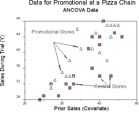
Note that we have 20 stores in each of two groups (Promo = 1; Control = -1) for a total of 40 stores. Let's take a peek at the data.

We want to know if the promotional has an effect on sales. From SAS PROC MEANS, we find that:

	Dependent Variable		Covariate
Group	Mean	SD	Mean	SD
Promo	39.25	5.98	35.60	6.30
Control	36.75	6.46	35.70	6.38

On the covariate (right columns), we find that the means and SDs are similar for both groups. On the dependent variable (left columns), the mean of sales is about 2.5 points higher for the promotional group than for the control group. Will this be a significant difference? ANOVA "decides" whether a difference is significant by looking at the mean difference in light of the SD and the sample size, N. In this problem, our mean difference is a little less that 1/2 standard deviation.

Well, we can do simple ANOVA without the covariate (that is, Y = a + b₁G). If we do, we find that the model has 1 df, with a sum of squares of 62.50, the error term has 38 df, with a sum of squares of 1473.5. Our F is 1.61, which is not significant (p = .21), and R² is .04.

But we know that lots of the variance in Y is due to location, management and labor effects. We can use prior sales to adjust or control for this. We start ANCOVA by looking for the interaction between the treatment and covariate. If we use PROC REG, we get the following results:

 

 

Model:	F=29.78	p < 1	R2 =.71
Variable	DF	Par Est	SE	T	P
Intercept	1	8.69	3.24	2.68	.01
G	1	1.13	3.24	.35	.73
X	1	.82	.09	9.18	.01*
GX	1	4	.09	.05	.96

As you can see, the model is significant and has a substantial R². The interaction term is not significant, so we can drop that term and revise our estimates, thus:

Model:	F=45.90	p < 1	R2 =.71
Variable	DF	Par Est	SE	T	P
Intercept	1	8.69	3.20	2.72	.01*
G	1	1.29	.55	2.37	.02*
X	1	.82	.09	9.30	1*

Note that both terms are significant. This means that the promotional has an effect that can be detected after removing the variance due to pre-existing differences in sales among stores within cells. The resulting regression model is one with two parallel lines - identical slopes but different intercepts.

I use PROC GLM rather than PROC REG for this kind of analysis. See the SAS lab manual for a description.

Recap: Our ANCOVA results thus far indicate that there is an effect of the promotional on sales. We can compute the regression lines for the two groups from the results of the REG procedure. Our equation:

Y' = 8.69+1.29G + .82X

We are using the common regression coefficient, b_c, which in this case is .82. The b for the group factor modifies the global intercept. For the promotional group, the value of G is 1, so for that group,

a_promo = 8.69+1.29 = 9.98, so for this group, the regression line is Y' = 9.98+.82X

For the control group, the value of G is -1, so for that group,

a_control = 8.69-1.29 = 7.4, so for this group, the regression line is Y' = 7.4+.82X.

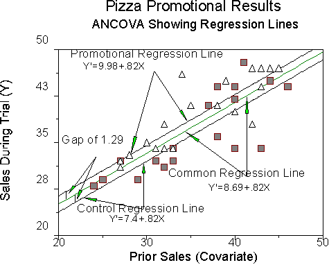
Recall that our regression from ANCOVA was Y' = 8.69+1.29G+.82X. Note that the slope for all three regression lines is .82. Note that the intercept of the common line is 8.69, which is the value of a. Note that the gap between each group and the common line is 1.29, which is the value of b for the G term.

Adjusted Means

When analysis of covariance is appropriate, we can adjust the means of the groups on Y for differences in X.

[Technical note: ANCOVA is appropriate when in addition to the ordinary assumptions of regression (approximate normality, homoscedasticity, linearity), we also have

1. the appropriateness of the common regression coefficient b_c assumption firmly supported by the data (b_c is the slope in the model with G and X but not GX in it; the test for GX supports the common slope b_c ) and
2. b_c is also large enough to make a difference (R² increases by about .10 by including the covariate over the model with the treatment only-- the correlation between X and Y needs to be about .30 for the covariate to do much for you. In our promotional example, r = .82.]

 

 

 

Back to adjusting means. The adjustment is:

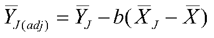
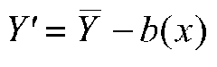
where is the adjusted mean of Group J on the DV, is the mean of Group J on the DV, b is b_c, the common slope, is the mean of Group J on the covariate, and is the grand mean of the covariate, that is, the mean on the covariate over all groups. Note that the formula for adjustment is just like the formula for predicting raw values (not means) in deviation score form, that is,

In our example, the data are

	X	Y
Grand Mean	35.65	38
Promo Mean	35.6	39.25
Control Mean	35.7	36.75

The adjusted means are

For the promotion group:

=39.25-.82(35.6-35.65) = 39.291.

For the control group:

= 36.75-.82(35.7-35.65) = 36.709.

Note that the adjusted means are slightly farther apart than the raw means; the promo group's mean is raised slightly and the control mean is lowered slightly. The reason for the adjustment is that the control group started out slightly richer, with better locations and/or more talented people than did the promotional group. ANCOVA can adjust for this difference. If we had done the instructional study in research methods, and found that at the start one group was smarter than the other was, we make an analogous adjustment for cognitive ability. Note that in both cases we randomly assigned people to treatments, so we expect minor adjustments only.

We can test for the differences among the adjusted means, too. There are some really ugly formulas to compute F for the difference. But we won't be using them because it turns out that testing for the difference between adjusted means is tantamount to (my favorite Pedhazur phrase) testing the difference between intercepts of regression lines that share a common slope. Testing for the difference between intercepts turns out to be the same as testing for the difference in b weights for the coded vectors that represent group membership. You remember that the b weight(s) for the G variable adjust the grand intercept up or down for each group, so the b weights amount to differences in intercepts. We can test for the significance of the difference between b weights in the same equation using a method we discussed early on. This method rests on the sampling covariance matrix of the b weights.

Fortunately for us, SAS will do this for us. In our example, I used the code:

 

Code	Meaning
proc glm;	Invoke the general linear models procedure
class g;	Variable G is categorical
model y = g x;	Regression model for ANCOVA
lsmeans g/ pdiff;	Give me least squares means (adjusted means) for variable G and test for their difference returning the probability for H0 that the means are equal.