TheResonant Filter Demoswith Positive Impact   NSFDUE 9952306

 
Objective: To model and analyze the behavior of a resonant filter, including the solution of a second-order, constant coefficient differential equation, the notions of a transient and a steady state solution, and the idea of resonance.

Level: Sophomore/Junior/Senior in a Differential Equations or a Mathematical Modeling course.

Prerequisites: Familiarity with techniques for solving second order differential equations (forexample from Boyce & DiPrima, (6th ed.) Sections 3.8 & 3.9 or Zill (7th ed), Chapter5). Acquaintance with basic circuit elements as discussed in a first course indifferential equations. An introduction to numerical solution of differentialequations would be helpful. 

Platform: A PC; custom software (developed using C++) is included.

Instructor'sNotes:

The resonant filter is a circuit element containing a resistor with resistance R, a capacitor with capacitance C, an inductor with inductance L and a voltage source. Its response can be modeled by a second-order,  constant-coefficient, non-homogeneous second order differential equation

where q(t) is the charge on the capacitor attime t and V_in(t) is the (known) voltage from the inputsource.   The equation can be reforumlated in terms of current, i(t),using the relation that i'(t) = q(t).  Differentiating, we obtain anequivalent equation in terms of the current in the circuit,

.

Let V_out(t) represent the voltagedrop across the resistor.  The relationship between the voltage and currentis given by V_out(t) = R i(t).  Thus, the second orderdifferential equation equation, represented in terms of V_out is

.

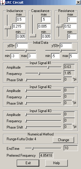
A program has been developed which takes as parameters the circuit elements, the source,and the initial conditions.  This program provides an interactive utilityfor a numerical simulation of the effect on the output by varying the parametersand the input signal.  

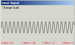
The program displays three components; the control panel, a graph of the input signal, and a graph of the output signal,represented by y(t). These are displayed in Figure 1.  

	Figure 1. Simulation of RLC filter with  R = 0.52, L = 0.215, C = 0.215, y(0) = 1, y'(0) = 0, and input signal .

Values for L, C, and Rare controlled by sliders.  Initial data are controlled by user input andthere are options for setting the viewing scale.  Three input signals ofthe form are allowed with controls for amplitude A, frequency,and phase shift . The initial value problem is solved using a choice of the fixed step size FourthOrder Runge-Kutta algorithm or the variable step size Runge-Kutta-Fehlbergalgorithm and the output function is graphed.  Each numerical routineprovides user control over step size.  A slider controls the end time andthe preferred frequency for the filter is calculated and displayed.

The accompanying help file, accessible by clicking the help button on the control panel, provides detailed instructions. (To see the help file .)

DEMO 1:  A basic demo involvessimply illustrating the solution to an initial value problem that models theresonant filter with one input signal.  Holding all parameters fixed exceptone, it is easy to investigate the effect on the output signal from changing thevalue of one of the physical parameters.  Such an experiment is shown inFigure 2.

	Figure 2.  Effect on output from varying C.

Aside from showing the numerically computed solution to the second order differential equationthat describes the resonant filter, there are three other useful demonstrations that this software canfacilitate.

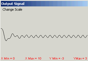
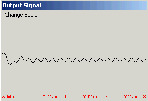
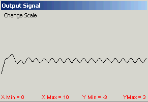
DEMO 2:  Solutions of a second order differential equation with constant coefficients and a sinusoidal forcingfunction decompose into two  components--a transient solution and a steady state solution. Simply sliding the bars for the initial data shows quite clearly the presence of a transient solution that depends on the initial data, and a steady state solution that is unaffected by changes in the initial data. Figure 3 shows the output signal for an RLC filter with R = 0.52, L= 0.215, C = 0.215, y(0) = 1,
y'(0) = 0, and input signal obtained by varying the initial conditions.  Observe the initial transientsolution and the steady state that does not change.

y(0) = 1, y'(0) = 0

y(0) = .5, y'(0) = 0

y(0) = -1, y'(0) = 2

Figure 3.  Effect on output from varying initial conditions.

DEMO 3:  This demo is useful forillustrating the phenomenon of resonance in an electrical device.  Althoughresonance is undesirable in many mechanical systems, such as a spring masssystem, many electrical devices such as radios would not function properlywithout the phenomenon of resonance.

Choose an input signal with a certainfrequency.  Fix the resistance and inductance.  Slide the capacitanceslider and observe the changes in the output curve as the preferred frequencychanges. Notice that the amplitude of the steady state signal is largest whenthe preferred frequency is close to the frequency of the input signal.  Wecan think of the capacitor as a tuner.

We can use the software to simulate aprimitive radio.  Assume that volume is roughly proportional to amplitudeand suppose we wish to pick up a radio station at a particular frequency (theinput frequency).  By adjusting the capacitor so that the amplitude is thehighest (this will occur when the preferred frequency is the same as the inputfrequency), we have simultaneously tuned in the station broadcasting at ourpreferred frequency and tuned out stations broadcasting at other frequencies.

DEMO 4:  Choosethree different input signals with different frequencies. Set the resistance toa low value, and slide either the inductance or capacitance values so that thepreferred frequency varies across the frequencies of your input signals. Youwill be able to visually pick out the frequencies that correspond to the inputfrequencies. It is another nice demonstration of a primitive method for tuning aradio.

In a course on scientific simulation, we had students construct a program like this. They were given tables of data formed by the sum of periodic signals and used their program to determine the frequencies of the original signals.

Material Included:

A zipped file with all requisite material is available; see below. This file contains the program, which should run on any recent PC, the help file which describes the program interface as well as the mathematical details of the model and the resonance phenomenon. Also included is a complete commented source code for those who wish to modify the program. There is no installation process; you need only unzip the package in a convenient directory.

To download the zipped file .

Once the files have been extracted, theutility is the executable file entitled LRC Circuit.exe.  To run theprogram, double click the program icon. 

This software can be used either as a classroom demonstration or in a lab situation. It is recommended that if you use this with students in a lab that you prepare a handout of experiments for students to perform and report on.

Other Resource:

is a java applet that illustrates resonance in an RLC circuit.  

References:

Davis, Paul, Differential Equations forMathematics, Science, and Engineering, Prentice Hall, 1992.

Edwards, C. Henry and David E. Penney, Differential Equations:  Computing and Modeling, Second Edition, Prentice Hall, 2000.

Boyce, William E. and Richard C. Diprima, ElementaryDifferential Equations, 6th Edition, John Wiley & Sons, 1996.

Zill, Dennis G., AFirst Course in Differential Equations with Modeling Applications, 7thEdition, Brooks-Cole, 2000.

---

Credits: This demo was submitted by 

Michael O'Leary

Towson University

and is included in Demoswith Positive Impact with his permission. The work of Michael O'Learywas supported by the National Science Foundation, under grant DUE 9952625.

---